One dimensional sieve introduction: Difference between revisions
No edit summary |
|||
| (41 intermediate revisions by the same user not shown) | |||
| Line 1: | Line 1: | ||
[http://cmpdartsvr3.cmp.uea.ac.uk/wiki/BanghamLab/index.php/MSER%27s_and_Connected_sets#One_dimensional_signals Return to MSERs and extrema]<br><br> | [http://cmpdartsvr3.cmp.uea.ac.uk/wiki/BanghamLab/index.php/MSER%27s_and_Connected_sets#One_dimensional_signals Return to MSERs and extrema]<br><br> | ||
Matlab function IllustrateSIV_1 illustrates how MSERs (maximally stable extremal regions) and sieves are related. We start with one dimensional signals before moving to two dimensional images and three dimensional volumes. | =<span style="color:Chocolate">1D Signals to MSERs and granules</span>= | ||
A Matlab function IllustrateSIV_1.m illustrates how MSERs (maximally stable extremal regions) and sieves are related. We start with one dimensional signals before moving to two dimensional images and three dimensional volumes.<br><br> | |||
The information lies in the pattern of pulses. Each pulse is characterised by a position, length (scale) and amplitude. The goal is to find maxima that persist over a number of scales - i.e. they are stable.<br><br> | |||
{| border="0" cellpadding="5" cellspacing="5" 3D extrema thumb.gif | |||
|- valign="top" | |||
|width="20%"| <!-- [[Image:IllustrateSIV_1_01_thumb.gif|140px|IllustrateSIV 1 01 thumb]]--> | |||
|'''Consider a signal''', <math>X</math><br> | |||
X=getData('PULSES3WIDE') | |||
>blue X=0 5 5 0 0 1 1 4 3 3 2 2 1 2 2 2 1 0 0 0 1 1 0 3 2 0 0 0 6 0 0 | |||
|} | |||
{| border="0" cellpadding="5" cellspacing="5" | {| border="0" cellpadding="5" cellspacing="5" | ||
|- valign="top" | |- valign="top" | ||
|width=" | |width="50%"| <math>X</math> has three one-sample-wide maxima (<math>M^1_8</math> , <math>M^1_{24}</math> , <math>M^1_{29}</math> ), two two-sample-wide maxima (<math>M^2_{14}</math> , <math>M^2_{21}</math>) some of which, when removed, will persist as larger scale maxima, e.g. <math>M^1_{24}</math> will become two samples wide as the peak is clipped off. | ||
|''' | |[[Image:IllustrateSIV_1_02.png|400px]] | ||
X= | |} | ||
> | |||
=<span style="color:Chocolate">Filter</span>= | |||
====<span style="color:SaddleBrown">Linear</span>==== | |||
{| border="0" cellpadding="5" cellspacing="5" | |||
|- valign="top" | |||
|width="50%"| A linear Gaussian filter with <math>\sigma=2</math> attenuates extrema without introducing new ones. The signal is simpler but has blurring made large scale information more difficult to read? | |||
|[[Image:GaussianSmoothedSigma2.png|350px|Gaussian filtered]] | |||
|} | |||
h=fspecial('Gaussian',9,2); | |||
Y=conv(X,(h(5,:)/sum(h(5,:))),'same'); | |||
====<span style="color:SaddleBrown">Non-linear: the starting point for MSER's</span>==== | |||
{| border="0" cellpadding="5" cellspacing="5" | |||
|- valign="top" | |||
|width="50%"| '''A low-pass''' 'o' sieve scale 1 (non-linear filter underpinning the MSER algorithm) can remove scale 1 maxima. The result is shown in red, extrema at <math>M^1_8</math> , <math>M^1_{24}</math> , <math>M^1_{29}</math> have been removed. There is no blur. The remaining signal is unchanged. | |||
|[[Image:IllustrateSIV_1_03.png|400px|'o' non-linear filter (sieve)]] | |||
|} | |||
scaleA=1; | |||
Y1=SIVND_m(X,scaleA,'o'); | |||
{| border="0" cellpadding="5" cellspacing="5" | |||
|- valign="top" | |||
|width="50%"| Scale 2 maxima are removed next using the 'o' sieve scale 2. The result is shown in green. Extrema at <math>M^2_{14}</math> , <math>M^2_{21}</math> have been removed. Still no blur and what remains is unchanged. | |||
|[[Image:IllustrateSIV_1_04.png|400px|'o' non-linear filter (sieve)]] | |||
|} | |||
scaleB=2; | |||
Y2=SIVND_m(X,scaleB,'o'); | |||
{| border="0" cellpadding="5" cellspacing="5" | |||
|- valign="top" | |||
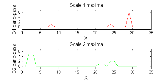
|width="50%"| '''A high-pass''' 'o' sieve scale 1 shows the extrema that have been removed. In red the scale 1 extrema at <math>M^1_8</math> , <math>M^1_{24}</math> , <math>M^1_{29}</math> have been removed. In green extrema of scale 2 are shown. ''In the sieve terminology these are granules.'' Think of grading gravel using sieves, large holes let through large grains and small holes let through small grains. Here scale is measured as length. If granules don't fit they don't get through - unlike linear filters which leak. | |||
|[[Image:IllustrateSIV_1_05.png|400px|'o' non-linear filter (sieve)]] | |||
|} | |||
red=double(X)-double(Y1); | |||
green=double(Y1)-double(Y2); | |||
====<span style="color:SaddleBrown">Repeat over scales 0 to 15</span>==== | |||
{| border="0" cellpadding="5" cellspacing="5" | |||
|- valign="top" | |||
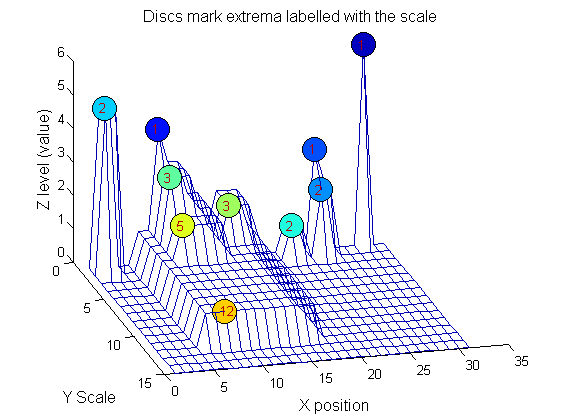
|width="50%"| Increasing the scale (towards the front) removes extrema of increasing length. The algorithm cannot create new maxima (it is an 'o' sieve) it is, therefore, scale-space preserving. | |||
|[[Image:Replacement IllustrateSIV 1 07.png|400px|'o' non-linear filter (sieve)]] | |||
|} | |||
YY=ones([length(X),1+maxscale]); | |||
for scale=0:maxscale | |||
Y2=SIVND_m(Y1,scale,'o',1,'l',4); | |||
YY(:,scale+1)=Y2'; | |||
Y1=Y2; <span style="color: Green">% each stage of the filter (sieve) is idempotent</span> | |||
end | |||
====<span style="color:SaddleBrown">Label the granules</span>==== | |||
{| border="0" cellpadding="5" cellspacing="5" | |||
|- valign="top" | |||
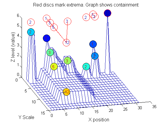
|width="50%"|We can create a data structure that captures the properties of each granule. The number in each disc indicates the granule scale. Each cell in the PictureElement field has a list of indexes recording the granule position (<math>X</math>). (In 1D this is best done run-length coded but this code is designed to also work in 2D.) | |||
|[[Image:IllustrateSIV_1_08.png|400px|'o' non-linear filter (sieve)]] | |||
|} | |||
g=SIVND_m(X,maxscale,'o',1,'g',4); | |||
g = Number: 10 | |||
area: [1 1 1 2 2 2 3 3 5 12] | |||
value: [6 1 1 2 5 1 1 1 1 1] | |||
level: [6 4 3 2 5 1 3 2 2 1] | |||
deltaArea: [5 2 1 7 3 12 2 2 7 19] | |||
last_area: [6 3 2 9 5 14 5 5 12 31] | |||
root: [29 8 24 24 2 21 8 14 8 8] | |||
PictureElement: {1x10 cell} | |||
g.PictureElement | |||
Columns 1 through 9 | |||
[29] [8] [24] [2x1 double] [2x1 double] [2x1 double] [3x1 double] [3x1 double] [5x1 double] [12x1 double] | |||
====<span style="color:SaddleBrown">Tracing the granules through scale-space identifies candidate MSER's</span>==== | |||
{| border="0" cellpadding="5" cellspacing="5" | |||
|- valign="top" | |||
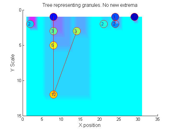
|width="50%"|The granules contain all the information in the signal. The tree illustrates the relationship between granules. The granules at <math>X=8</math> (scales 1, 3, 5, 12) indicates a region that is stable over scale. Likewise at <math>X=24</math> (scales 1, 2). One might argue that the latter is the less stable. | |||
[[Image:IllustrateSIV_1_10.png|250px|'o' non-linear filter (sieve)]] | |||
|[[Image:IllustrateSIV_1_09.png|400px|'o' non-linear filter (sieve)]] | |||
|} | |} | ||
=<span style="color:Chocolate">We have candidate 1D MSER's</span>= | |||
<span style="color:SaddleBrown">'''Which is the ''most stable''?'''<br><br> | |||
This is a pragmatic judgement. Parameters might include</span> | |||
#<span style="color:SaddleBrown">how stable over scale (length)</span> | |||
#<span style="color:SaddleBrown">amplitude (value or level)</span> | |||
#<span style="color:SaddleBrown">a vector of amplitude over scale</span> | |||
#<span style="color:SaddleBrown">proximity to others</span> | |||
=<span style="color:Chocolate">So far '''''maxima'''''. What about ''minima'' and more?</span>= | |||
The filter (sieve) that finds maxima is a connect-set ''opening'' ('o' sieve). A 'c' sieve finds the connected-set closing, or minima. To work with minima we could: | |||
*invert the signal, process it, and invert it back. | |||
*OR, in this case, we could substitute a min for a max within SIVND_m. | |||
YY=ones([length(X),1+maxscale]); | |||
for scale=0:maxscale | |||
Y2=SIVND_m(X,scale,'c',1,'l',4); | |||
YY(:,scale+1)=Y2'; | |||
Y1=Y2; % each stage of the filter (sieve) is idempotent | |||
end | |||
g=SIVND_m(X,maxscale,'c',1,'g',4); | |||
{| border="0" cellpadding="5" cellspacing="5" | {| border="0" cellpadding="5" cellspacing="5" | ||
|- valign="top" | |- valign="top" | ||
[[Image: | |width="50%"|Closing sieve 'c' sieve. To make it clearer the 'FaceColor' is 'flat' and the graph is placed at the bottom. To find minima at ALL scales it would be necessary to go to scales greater than 15.<br><br> | ||
<span style="color:Chocolate">'''Which is better for finding 1D MSER's, 'o' or 'c'?'''</span> | |||
*It depends on the data | |||
*Further alternative operators include 'M', 'N' and 'm' which might be better still (to be discussed elsewhere). | |||
|[[Image:Illustrate_c_SIV_1_09.png|400px|'o' non-linear filter (sieve)]] | |||
|} | |} | ||
This implementation also maintains ''lists of both maxima and minima'' throughout because there can be value in using the combined operators M, N, m | |||
switch type | |||
case {'o'} % opening, merge all maximal runs of less than scale with their nearest value | |||
data=ND_connected_set_merging(data,scale,type,verbose); | |||
case {'c'} % closing, merge all minima runs of less than scale with their nearest value | |||
data=ND_connected_set_merging(data,scale,type,verbose); | |||
case {'C'} % closing, invert-open-invert | |||
data.workArray=uint8(-double(data.workArray)+256); | |||
data.value=uint8(-double(data.value)+256); | |||
data=ND_connected_set_merging(data,scale,'o',verbose); | |||
data.workArray=uint8(-double(data.workArray)+256); | |||
data.value=uint8(-double(data.value)+256); | |||
case 'M' % Open close | |||
data=ND_connected_set_merging(data,scale,'o',verbose); | |||
data=ND_connected_set_merging(data,scale,'c',verbose); | |||
case 'N' % Close open | |||
data=ND_connected_set_merging(data,scale,'c',verbose); | |||
data=ND_connected_set_merging(data,scale,'o',verbose); | |||
case 'm' % recursive median | |||
data=ND_connected_set_rmedian(data,scale,'m',verbose); | |||
otherwise | |||
error('type not recognised it should be (m, o, c, C, M or N)'); | |||
end | |||
Latest revision as of 15:55, 3 January 2014
1D Signals to MSERs and granules
A Matlab function IllustrateSIV_1.m illustrates how MSERs (maximally stable extremal regions) and sieves are related. We start with one dimensional signals before moving to two dimensional images and three dimensional volumes.
The information lies in the pattern of pulses. Each pulse is characterised by a position, length (scale) and amplitude. The goal is to find maxima that persist over a number of scales - i.e. they are stable.
Consider a signal, <math>X</math>X=getData('PULSES3WIDE')
>blue X=0 5 5 0 0 1 1 4 3 3 2 2 1 2 2 2 1 0 0 0 1 1 0 3 2 0 0 0 6 0 0
|
Filter
Linear
| A linear Gaussian filter with <math>\sigma=2</math> attenuates extrema without introducing new ones. The signal is simpler but has blurring made large scale information more difficult to read? | 
|
h=fspecial('Gaussian',9,2);
Y=conv(X,(h(5,:)/sum(h(5,:))),'same');
Non-linear: the starting point for MSER's
scaleA=1;
Y1=SIVND_m(X,scaleA,'o');
scaleB=2;
Y2=SIVND_m(X,scaleB,'o');
red=double(X)-double(Y1);
green=double(Y1)-double(Y2);
Repeat over scales 0 to 15
| Increasing the scale (towards the front) removes extrema of increasing length. The algorithm cannot create new maxima (it is an 'o' sieve) it is, therefore, scale-space preserving. | 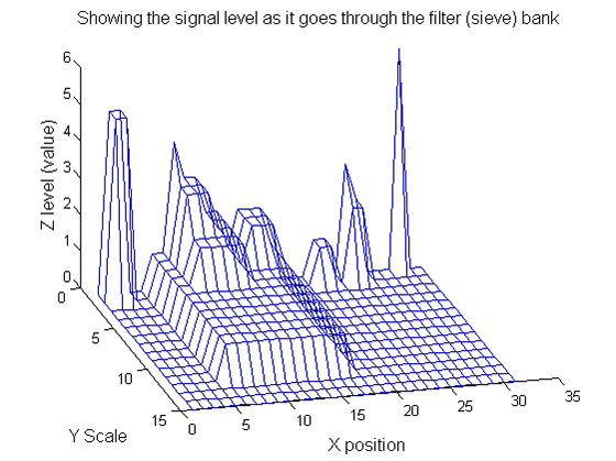
|
YY=ones([length(X),1+maxscale]);
for scale=0:maxscale
    Y2=SIVND_m(Y1,scale,'o',1,'l',4);
    YY(:,scale+1)=Y2';
    Y1=Y2; % each stage of the filter (sieve) is idempotent
end
Label the granules
g=SIVND_m(X,maxscale,'o',1,'g',4);
g =   Number: 10
             area: [1 1 1 2 2 2 3 3 5 12]
            value: [6 1 1 2 5 1 1 1 1 1]
            level: [6 4 3 2 5 1 3 2 2 1]
        deltaArea: [5 2 1 7 3 12 2 2 7 19]
        last_area: [6 3 2 9 5 14 5 5 12 31]
             root: [29 8 24 24 2 21 8 14 8 8]
   PictureElement: {1x10 cell}
g.PictureElement
Columns 1 through 9
[29] [8] [24] [2x1 double] [2x1 double] [2x1 double] [3x1 double] [3x1 double] [5x1 double] [12x1 double]
Tracing the granules through scale-space identifies candidate MSER's
We have candidate 1D MSER's
Which is the most stable?
This is a pragmatic judgement. Parameters might include
- how stable over scale (length)
- amplitude (value or level)
- a vector of amplitude over scale
- proximity to others
So far maxima. What about minima and more?
The filter (sieve) that finds maxima is a connect-set opening ('o' sieve). A 'c' sieve finds the connected-set closing, or minima. To work with minima we could:
- invert the signal, process it, and invert it back.
- OR, in this case, we could substitute a min for a max within SIVND_m.
YY=ones([length(X),1+maxscale]);
for scale=0:maxscale
    Y2=SIVND_m(X,scale,'c',1,'l',4);
    YY(:,scale+1)=Y2';
    Y1=Y2; % each stage of the filter (sieve) is idempotent
end
g=SIVND_m(X,maxscale,'c',1,'g',4);
This implementation also maintains lists of both maxima and minima throughout because there can be value in using the combined operators M, N, m
       switch type
           case {'o'} % opening, merge all maximal runs of less than scale with their nearest value
               data=ND_connected_set_merging(data,scale,type,verbose);
           case {'c'} % closing, merge all minima runs of less than scale with their nearest value
               data=ND_connected_set_merging(data,scale,type,verbose);
           case {'C'} % closing, invert-open-invert
               data.workArray=uint8(-double(data.workArray)+256);
               data.value=uint8(-double(data.value)+256);
               data=ND_connected_set_merging(data,scale,'o',verbose);
               data.workArray=uint8(-double(data.workArray)+256);
               data.value=uint8(-double(data.value)+256);
           case 'M' % Open close
               data=ND_connected_set_merging(data,scale,'o',verbose);
               data=ND_connected_set_merging(data,scale,'c',verbose);
           case 'N' % Close open
               data=ND_connected_set_merging(data,scale,'c',verbose);
               data=ND_connected_set_merging(data,scale,'o',verbose);
           case 'm' % recursive median
               data=ND_connected_set_rmedian(data,scale,'m',verbose);
           otherwise
               error('type not recognised it should be (m, o, c, C, M or N)');
       end


