"Evolutionary Paths Underlying Flower Color Variation in Antirrhinum"
Abstract
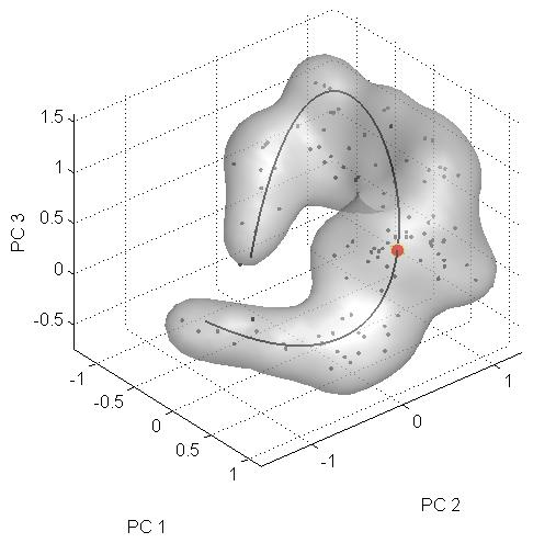
To understand evolutionary paths connecting diverse biological forms, we defined a three-dimensional genotypic space separating two flower color morphs of Antirrhinum. A hybrid zone between morphs showed a steep cline specifically at genes controlling flower color differences, indicating that these loci are under selection. Antirrhinum species with diverse floral phenotypes formed a U-shaped cloud within the genotypic space. We propose that this cloud defines an evolutionary path that allows flower color to evolve while circumventing less-adaptive regions. Hybridization between morphs located in different arms of the U-shaped path yields low-fitness genotypes, accounting for the observed steep clines at hybrid zones.
The Manuscript
“Evolutionary Paths Underlying Flower Color Variation in Antirrhinum”, A. C. Whibley, N. B. Langlade, C. Andalo, A. I. Hanna, J. A. Bangham, and E. S. Coen
Downloading the Project and AAMToolbox
The project used to create the figures in the manuscript, together with the Matlab toolbox that manages the project and the manuscript can be downloaded here. (This contains version 6.5 of the AAMToolbox)
To create the figures shown in the manuscript “Evolutionary Paths Underlying Flower Color Variation in Antirrhinum”, A. C. Whibley, N. B. Langlade, C. Andalo, A. I. Hanna, J. A. Bangham, and E. S. Coen, Science, 313:963-966, 2007, please follow the instructions below.
These figures were created using Matlab 2006b version 7.3.0.267 running on Windows XP.
Installing the AAMToolbox
To install the toolbox, unzip the zip file you downloaded from the section above (some unzippers think the file is locked, WinZip and WinRar seem to handle it just fine). In that folder you will find 2 folders, the first one will be the ‘AAMToolbox’ folder (this contains the Matlab files that run the toolbox). The second folder is named ‘PRJ_Science’. This is the project folder that contains all the data for the manuscript. To install the toolbox, from the Matlab prompt type
>>pathtool
Click the ‘Add with subfolders’ button and then select the AAMToolbox folder. Save your new path and return to Matlab. You have now installed the toolbox. REMEMBER, ANY CHANGES YOU MAKE TO THE TOOLBOX DIRECTORY WILL REQUIRE YOU TO RESET THE PATH USING PATHOOL.
Creating Figures
Figure 4 (f)

Firstly you must make sure that you have correctly installed the Toolshed from here. Secondly, you must have downloaded and saved the project PRJ_Science to your hard disk. If you have done these steps, then start Matlab. In matlab move to project directory PRJ_Science, from the Matlab prompt type
>>AAMToolbox
This will start the AAMToolbox and if you are in the correct directory you will be presented with the correct details for the project corresponding to this paper.
- Click the View Shape Space button.
- Click the Open button from the Group panel.
- Select SciencePaperGroups.mat and click Open.
- Click the Load button from the Group panel.
a dialog box with the text Loading Group Data, Please Wait.. will appear, when this dialog box closes you have loaded your groups.
- Select Tools->Units->Standard Deviations
- Click the Choose App. Axes button from the Display Options Panel
- Select PC's 1, 2 and 3 and click Ok
- Click the Choose Shape Axes button from the Display Options Panel
- Select PC's 1, 2 and 3 and click Ok
- Uncheck Group Labels from the Plot Options panel
- Set dx=30, dy=30 and dz=30 in the Surface Quantization panel
- Click the Fit Surface button from the Display Options Panel
a dialog box will appear telling you that the surface has been fitted, close this by clicking Ok.
- Check Iso-Surface box from the Plot Options panel
- Slide the Isosurface Level slider to 3 in the Isosurface Pane
- Bring the Appearance window to the front to see the surface.