Details on hydrophobicity plots: Difference between revisions
| (14 intermediate revisions by the same user not shown) | |||
| Line 1: | Line 1: | ||
[[MSER_and_Sieve_Details# | [[MSER_and_Sieve_Details#Applications | Back to MSERs etc]] | ||
=====<span style="color:Navy;">Trying to spot regions (lengths) that are up (hydrophobic) and down (hydrophilic)</span>===== | =====<span style="color:Navy;">Trying to spot regions (lengths) that are up (hydrophobic) and down (hydrophilic)</span>===== | ||
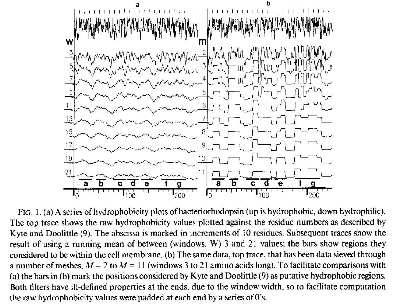
Left: Running mean (c.f Gaussian): <span style="color:blue;">no good</span>, Right: Median based Data-sieve: <span style="color:blue;">much better</span> | Left: Running mean (c.f Gaussian): <span style="color:blue;">no good</span>, Right: Median based Data-sieve: <span style="color:blue;">much better</span> | ||
[[Image:HydrophobicityPlot_Bacteriorhodopsin.png|700px]] | [[Image:HydrophobicityPlot_Bacteriorhodopsin.png|700px]] | ||
Bangham, J.A. (1988) Data-sieving hydrophobicity plots. Anal. Biochem. 174, 142–145< | <span style="color:Navy;">Bangham, J.A. (1988) Data-sieving hydrophobicity plots. Anal. Biochem. 174, 142–145</span><br> | ||
====Abstract==== | |||
= | <span style="color:Navy;">''Hydrophobicity plots provide clues to the tertiary structure of proteins (J. Kyte and R. F. Doolittle, 1982, J. Mol. Biol.157, 105; C. Chothia, 1984, Annu. Rev. Biochem.53, 537; T. P. Hopp and K. R. Woods, 1982, Proc. Natl. Acad. Sci. USA78, 3824). To render domains more visible, the raw data are usually smoothed using a running mean of between 5 and 19 amino acids. This type of smoothing still incorporates two disadvantages. First, peculiar residues that do not share the properties of most of the amino acids in the domain may prevent its identification. Second, as a low-pass frequency filter the running mean smoothes sudden transitions from one domain, or phase, to another. Data-sieving is described here as an alternative method for identifying domains within amino acid sequences. The data-sieve is based on a running median '''''and is characterized by a single parameter, the mesh size, which controls its resolution'''''. It is a technique that could be applied to other series data and, '''''in multidimensions, to images''''' in the same way as a median filter.''</span> | ||
For the data-sieve I used a cascade of medians which was a very inefficient implementation. Subsequently, I switched to a cascade of 1D recursive medians which also ''preserved scale space'' but was both ''quicker and idempotent''. | |||
====Fasman et al reviewed different hydrophobicity plots including the data-sieve==== | |||
[[Image:hydrophobicity_plots_Fasman.jpg|700px]]<br><br> | [[Image:hydrophobicity_plots_Fasman.jpg|700px]]<br><br> | ||
| Line 16: | Line 17: | ||
Left: Running mean (c.f Gaussian): <span style="color:blue;">no good</span>, Right: Median based Data-sieve: <span style="color:blue;">much better</span><br><br> | Left: Running mean (c.f Gaussian): <span style="color:blue;">no good</span>, Right: Median based Data-sieve: <span style="color:blue;">much better</span><br><br> | ||
These authors compared many different methods and <span style="color:blue;">concluded that the data-sieve was best</span>. However, they found a reason not to recommend it: | These authors compared many different methods and <span style="color:blue;">concluded that the data-sieve was best</span>. However, they found a reason not to recommend it: they didn't understand how it worked.<br><br> | ||
Well there you are then. Means verses medians.<br><br> | <span style="color:#A52A2A;">Well there you are then. Means verses medians.</span><br><br> | ||
'''Actually''', there are some simple computational issues here. At the time computers were only just becoming commonplace and they were not (by current standards) powerful. Computing a running mean is very easy. Choose a window size, ''n'', and start by adding up all the values in the first ''n'' samples to make ''S''. Divide by ''n'' and you have the first point. Now move along by one value - add the new value to ''S'', subtract the first (the outgoing) value from ''S'' and divide by ''n'' again. Add, subtract, divide: easy and the size of ''n'' does not matter. The median is harder, it requires a sort of some type. But I discovered a neat alternative, the recursive median ('m') sieve, indeed I found a family of such filter banks with different kernels 'o', 'c', 'M', 'N', and 'm' and called them all sieves. | |||
They are also trivial to compute in 1D. | |||
==Don't give up, get motivated== | ==Don't give up, get motivated== | ||
The good thing was that I was motivated to prove exactly how it worked and why it was so good - I moved to Computing Sciences and published everything in computing journals. Where computer scientists would find it - or not - think MSER literature.<br><br> | The good thing was that I was motivated to prove exactly how it worked and why it was so good - I moved to Computing Sciences and published everything in computing journals. Where computer scientists would find it - or not - think MSER literature.<br><br> | ||
I was | I was particularly excited about the possibility that the new set of scale-space preserving transforms might shine a new and different light on brain vision. Fourier transforms, wavelets, Gabor filters etc. may not always be the right light (OK I agree, the 'standard' explanations are very consistent with the evidence, but sometimes one should test and reject alternatives). I attended conferences on vision - the amazing Horace Barlow's retirement bash, the 6 month extravaganza: ''Computer Vision'' at the Isaac Newton Institute for Mathematical Sciences (University of Cambridge, United Kingdom) July to December, 1993. Organised by scientists that I greatly admire: David Mumford (Harvard), Andrew Blake, Brian Ripley (Oxford) etc. However, it was difficult. A typical remark was 'But mathematicians have shown that Gaussian Filter banks are unique ...' The focus then was on anisotropic diffusion.<br><br> | ||
I was <span style="color:blue;">proving</span> that | I was <span style="color:blue;">proving</span> that diffusion filters are not unique. <br><br> | ||
The non-linear filters I was describing held the promise of extremely useful properties in computer vision - as it turns out one example | The non-linear filters I was describing held the promise of extremely useful properties in computer vision - as it turns out one example would be the MSER's. Some of their success will be down to the front end processing preserving scale space. | ||
Latest revision as of 14:00, 30 July 2014
Trying to spot regions (lengths) that are up (hydrophobic) and down (hydrophilic)
Left: Running mean (c.f Gaussian): no good, Right: Median based Data-sieve: much better
 Bangham, J.A. (1988) Data-sieving hydrophobicity plots. Anal. Biochem. 174, 142–145
Abstract
Hydrophobicity plots provide clues to the tertiary structure of proteins (J. Kyte and R. F. Doolittle, 1982, J. Mol. Biol.157, 105; C. Chothia, 1984, Annu. Rev. Biochem.53, 537; T. P. Hopp and K. R. Woods, 1982, Proc. Natl. Acad. Sci. USA78, 3824). To render domains more visible, the raw data are usually smoothed using a running mean of between 5 and 19 amino acids. This type of smoothing still incorporates two disadvantages. First, peculiar residues that do not share the properties of most of the amino acids in the domain may prevent its identification. Second, as a low-pass frequency filter the running mean smoothes sudden transitions from one domain, or phase, to another. Data-sieving is described here as an alternative method for identifying domains within amino acid sequences. The data-sieve is based on a running median and is characterized by a single parameter, the mesh size, which controls its resolution. It is a technique that could be applied to other series data and, in multidimensions, to images in the same way as a median filter.
For the data-sieve I used a cascade of medians which was a very inefficient implementation. Subsequently, I switched to a cascade of 1D recursive medians which also preserved scale space but was both quicker and idempotent.
Fasman et al reviewed different hydrophobicity plots including the data-sieve

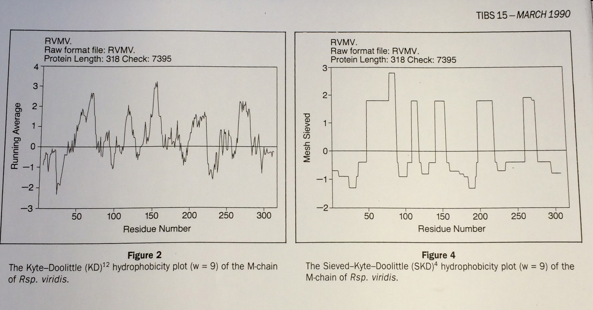
From Fasman and Gilbert "The prediction of transmembrane protein sequences and their conformation: an evaluation" in Trends in Biochemistry 15 pp 89:91
Left: Running mean (c.f Gaussian): no good, Right: Median based Data-sieve: much better
These authors compared many different methods and concluded that the data-sieve was best. However, they found a reason not to recommend it: they didn't understand how it worked.
Well there you are then. Means verses medians.
Actually, there are some simple computational issues here. At the time computers were only just becoming commonplace and they were not (by current standards) powerful. Computing a running mean is very easy. Choose a window size, n, and start by adding up all the values in the first n samples to make S. Divide by n and you have the first point. Now move along by one value - add the new value to S, subtract the first (the outgoing) value from S and divide by n again. Add, subtract, divide: easy and the size of n does not matter. The median is harder, it requires a sort of some type. But I discovered a neat alternative, the recursive median ('m') sieve, indeed I found a family of such filter banks with different kernels 'o', 'c', 'M', 'N', and 'm' and called them all sieves.
They are also trivial to compute in 1D.
Don't give up, get motivated
The good thing was that I was motivated to prove exactly how it worked and why it was so good - I moved to Computing Sciences and published everything in computing journals. Where computer scientists would find it - or not - think MSER literature.
I was particularly excited about the possibility that the new set of scale-space preserving transforms might shine a new and different light on brain vision. Fourier transforms, wavelets, Gabor filters etc. may not always be the right light (OK I agree, the 'standard' explanations are very consistent with the evidence, but sometimes one should test and reject alternatives). I attended conferences on vision - the amazing Horace Barlow's retirement bash, the 6 month extravaganza: Computer Vision at the Isaac Newton Institute for Mathematical Sciences (University of Cambridge, United Kingdom) July to December, 1993. Organised by scientists that I greatly admire: David Mumford (Harvard), Andrew Blake, Brian Ripley (Oxford) etc. However, it was difficult. A typical remark was 'But mathematicians have shown that Gaussian Filter banks are unique ...' The focus then was on anisotropic diffusion.
I was proving that diffusion filters are not unique.
The non-linear filters I was describing held the promise of extremely useful properties in computer vision - as it turns out one example would be the MSER's. Some of their success will be down to the front end processing preserving scale space.