Running example models and using a cluster
The purpose of these tutorials is to learn how to run the example growth simulations included in GFtbox. We will describe methods for running simulations locally (on your own computer) and remotely (on a computing cluster). It is assumed that you have already downloaded the GFtbox software and have Matlab installed.
Getting Started
The remainder of this page is split into five sub-tutorials, each building on the preceding parts.
1) Explaining the tools. In these tutorials, we will be using GFtboxCommand and ClusterMonitor. This section explains the purpose of these tools.
2) Computer or cluster? Here, we illustrate when and why you should use a computing cluster for your growth simulations, and conversely, when you should use your desktop computer.
3) Running a growth simulation for an example model. This section demonstrates how to use GFtboxCommand to run a growth simulation on your computer. The model used for the simulation is an example model included with the GFtbox.
4) Altering the simulation parameters. Following on from part 3, here we show how to adjust a simulation parameter within GFtboxCommand. Specifically, we alter the value of dt, the temporal resolution of the simulation, and show how it can be used to verify that the value specified in the published literature is reasonable.
5) Altering the model parameters. Finally, we demonstrate how a number of model parameters can be varied by specifying a range of values for each model argument. We show how the computationally expensive task of simulating all combinations of specified ranges can be processed more efficiently if a computer cluster is used via the ClusterMonitor tool.
1 Explaining the tools
GFtboxCommand
This is a command line version of the GFtbox. By command line, we mean that all program functions are operated via typed commands, without the GUI. Like GFtbox, GFtboxCommand is capable of running growth simulations of an interaction function, and allows the user to specify model and simulation parameters. Unlike GFtbox, this also allows the user to select ranges of values for a number of input parameters, and will automatically spawn multiple simulations which explore the various combinations of those parameters. This can be used to evaluate the effect of various parameters on the growth of a given model.
ClusterMonitor
Provides a graphical user interface for managing simulations running remotely on a computer cluster. Specifically, it allows you to see which projects are present and running on the cluster, to retrieve the completed projects, to generate images of the simulations at specified stages of growth, and to remove projects from the cluster. If you do not intend to use a computer cluster, then you will not need to use ClusterMonitor.
2 Computer or cluster?
In basic terms, a computing cluster is effectively a network of many computer processors (often hundreds), centrally managed by a queuing system. When a job is submitted to a cluster, the job is sent to a processor that is not being used, or queued until one becomes available. In contrast, a typical desktop computer will contain one processor, limiting the number of tasks that can be performed at any one time. Jobs which must be run independently and sequentially on a desktop computer can be executed in parallel on a cluster, greatly reducing the total time required to complete all of the jobs. Although the exact details of your cluster might vary from those described in the rest of these tutorials, we aim to illustrate the generic processes involved in using GFtbox on a cluster. We are happy to offer assistance, where possible, to setup GFtbox for your cluster, so please contact us if you have any queries.
Whilst the time savings offered by using a cluster can be significant, there is an overhead associated with returning the results to your personal computer. The total time to run 2 or more simulations on a cluster and to return the results will be less than running those simulations sequentially on one computer. Therefore, using a cluster is ideal for situations where you would like to run several simulations, such as to evaluate the effect of a range of parameters on a growth model. You are not advised to use a cluster for running single simulations, or where you would like to step through a simulation and change parameters in a more interactive fashion. In such circumstances, you are advised to run GFtbox or GFtboxCommand on your own computer.
The GFtbox GUI provides quick feedback about how the changes you have made to an interaction function have affected the growth simulation, as you can see the result of each simulation iteration as it completes. It is quick and easy therefore to see if you have dramatically changed the course of the growth simulation, and then to adjust the parameters according to your observations. This approach is well suited to the early stages of design, where you might wish to tweak some parameters to gauge whether or not they have had the desired effect. Or in the final stages, where you think your model is almost finalised, but where small adjustments are required. An alternative approach is to start many simulations, based upon your initial model and by making intelligent choices about which parameters to explore. This allows you to harvest many results, to quickly and easily overview them in their finalised form, or to select interesting-looking simulations and examine them more closely on your desktop computer, using GFtbox.
3 Running a growth simulation for an example model
This tutorial is aimed at running a growth simulation for one of the example interaction functions included with the GFtbox. The purpose of this exercise is to firstly demonstrate how simulations can be invoked using GFtboxCommand, and secondly to show how to reproduce experimental results (specifically, those published in Kennaway et al (2011)) given an interaction function.
Assuming Matlab is installed on your computer, and the latest GFtbox has been downloaded, you can add the GFtbox directory to Matlab's search path, which makes the toolbox accessible from any other path that you choose to work from. For a short tutorial on how to do this, please click here.
Once the GFtbox is added to Matlab, you are ready to run a growth simulation using GFtboxCommand. In this example, the model that we will simulate is called GPT_CASE_RST. Results generated using this model are published in Kennaway et al (2011). By running this simulation, we can confirm the results in the published literature and investigate the suitability of the various parameters.
3A - Running a simulation on your computer
The following command can be typed into Matlab to run a simulation of the GPT_CASE_RST interaction function, which contains three growth models: R, S and T. Three separate simulations are run sequentially on your computer, one for each model, each producing results corresponding to five intervals in the growth simulation.
       GFtboxCommand('Path','/GrowthToolbox/Models/Published/Kennaway-etal-2011/','Name','GPT_CASE_RST',...
       'Stages',[20 100 140 180 200],'modelname',[1:3]);
GFtboxCommand accepts input arguments as name and value pairs, e.g. 'modelname', [1:3] or 'Use','Cluster'. The argument names entered in the example above are: Path, Name, Stages and modelname.
The optional Path argument name refers to the location of the folder (or directory) on your computer where the model interaction function you wish to simulate is stored. Name, is the name of the folder itself. In this case, we are using the GPT_CASE_RST folder which is included in the GrowthToolbox. You may wish to copy this folder elsewhere, if you intend to make changes to the interaction function.
During a growth simulation, a mesh can be generated at each time step of the simulation, which provides a visual representation of the growth of the biological tissue, given the various parameters of growth specified by the interaction function and how they have changed over time. Put another way, the mesh shows exactly what the growing tissue actually looks like. Stages refers to the points in the simulation (measured in hours) at which meshes should be generated and saved. In this example, five stages of growth will be written to disk. These values are chosen to best capture the appearance of the tissue at important stages of the tissue growth.
The final argument name listed here is modelname. This is a model-specific argument, and in this case the GPT_CASE_RST interaction function contains three separate models for plant growth, allowing the desired model to be a selected. Here, the value [1:3] is specified, which is evaluated in the same way as entering [1 2 3]. This instructs GFtboxCommand to run three separate simulations, one for each of the growth models contained in the interaction function.
The function of every permissible argument is given by keying the following command into Matlab:
help GFtboxCommand
3B - Getting results from a completed simulation
1) - Generating images from a simulation you ran on your computer
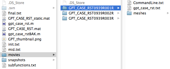
Once a growth simulation is completed, the project folder (GPT_CASE_RST, in our example) will contain another folder named "movies". Within movies, there are folders which contain results for the executed simulations. As was instructed in 3A, here we can see three folders corresponding to simulations for the three separate models. Within the first folder there are three items:
The mesh files contain vertices information regarding the shape of the growth model at a particular stage of growth, but are not visualisable in that form. In order to convert these mesh files into viewable images, we can execute the following command in Matlab:
       VMSreport('Path','/GrowthToolbox/Models/Published/Kennaway-etal-2011/','Project','GPT_CASE_RST',...
       'Experiment','All','flattentime',572.5,'morphogen','KPAR','SNAPFIG',true);
Where the Path and Project arguments have the same function as Path and Name in 3A, i.e. Path refers to the location of the project folder and Project is the name of the project folder itself.
Here we can see the generated images, including the command line arguments, for one of the simulations performed in 3A. Click on a thumbnail to view a larger image.
001commandline.png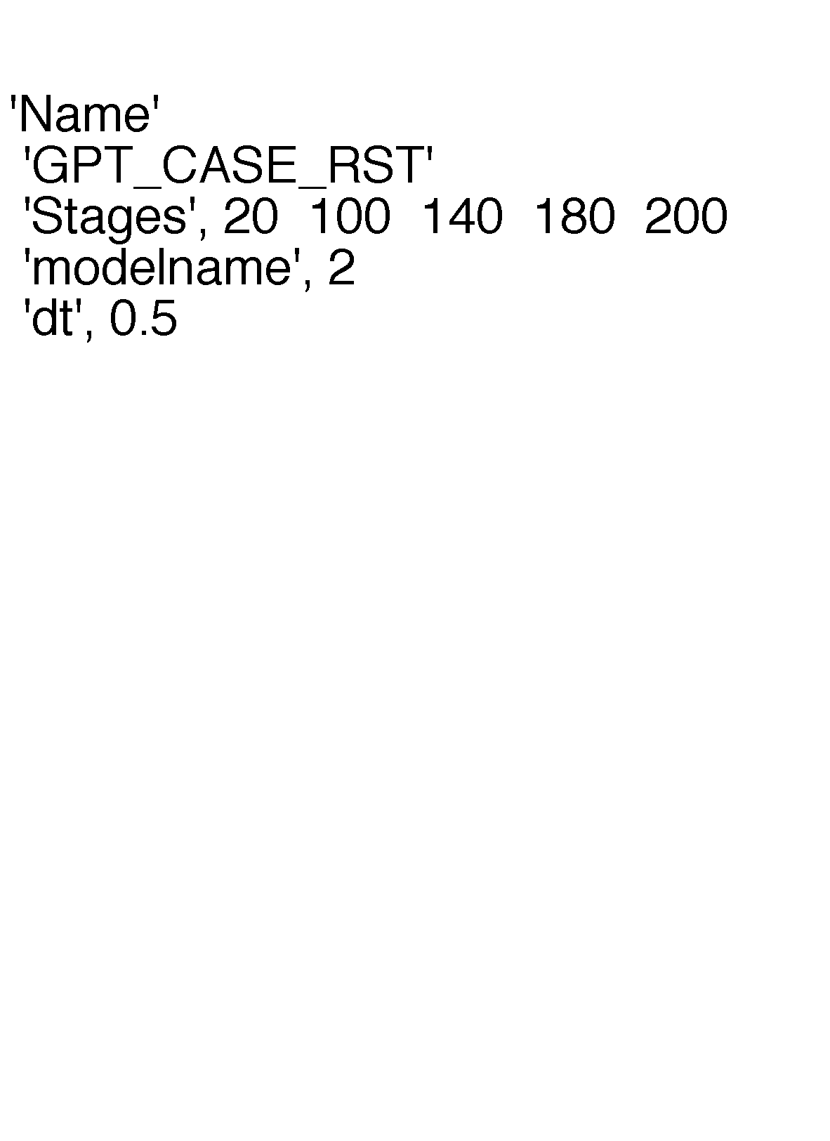
|
001GPT_CASE_RST_2 wild_.png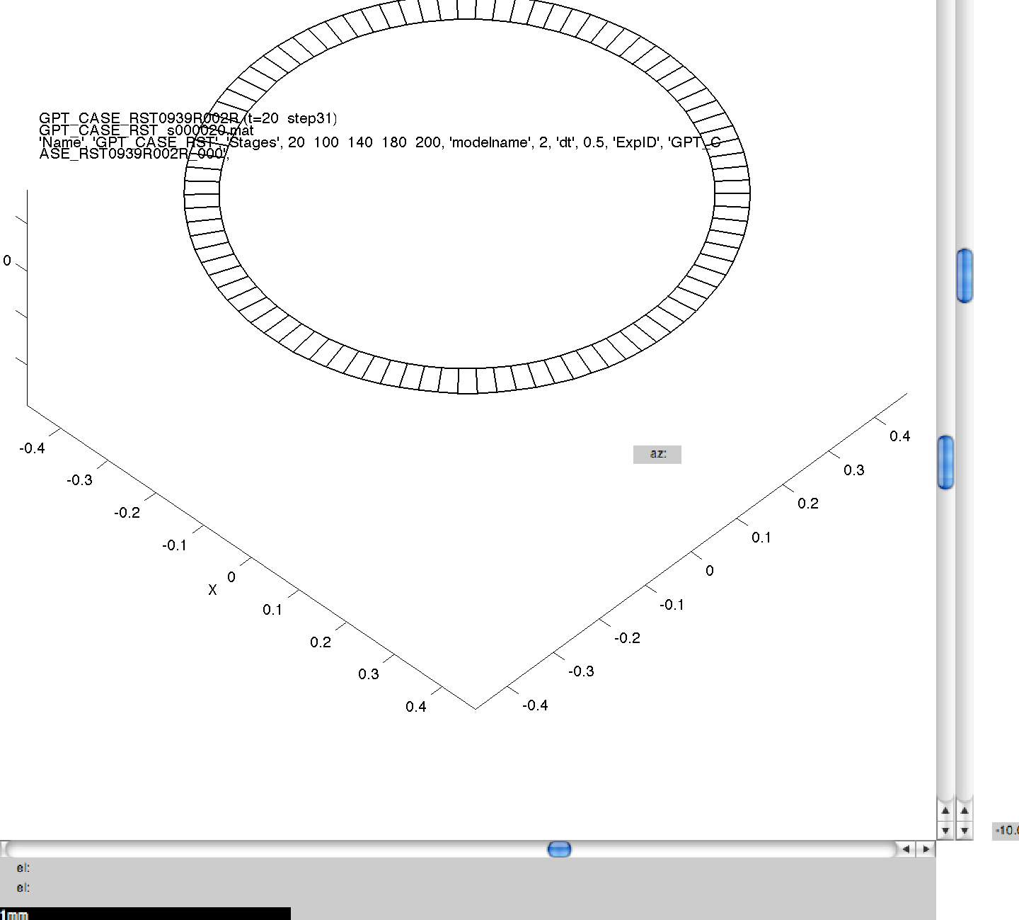
|
001GPT_CASE_RST_3 wild_.png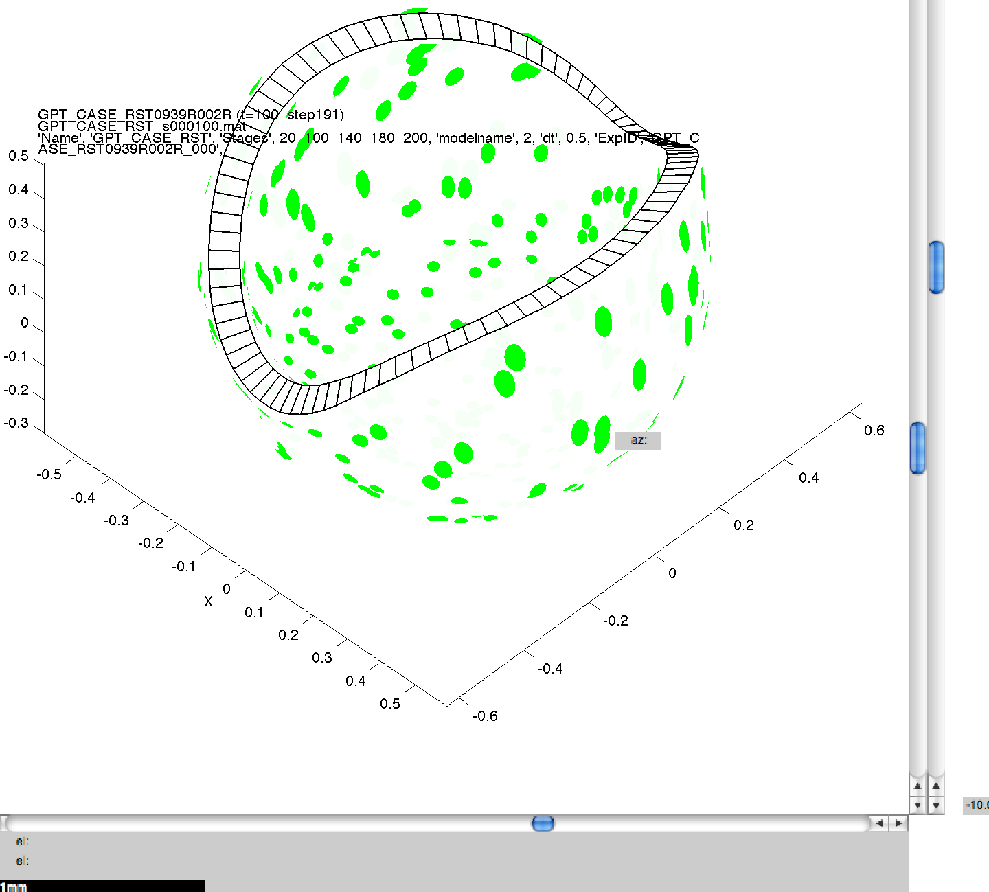
|
001GPT_CASE_RST_4 wild_.png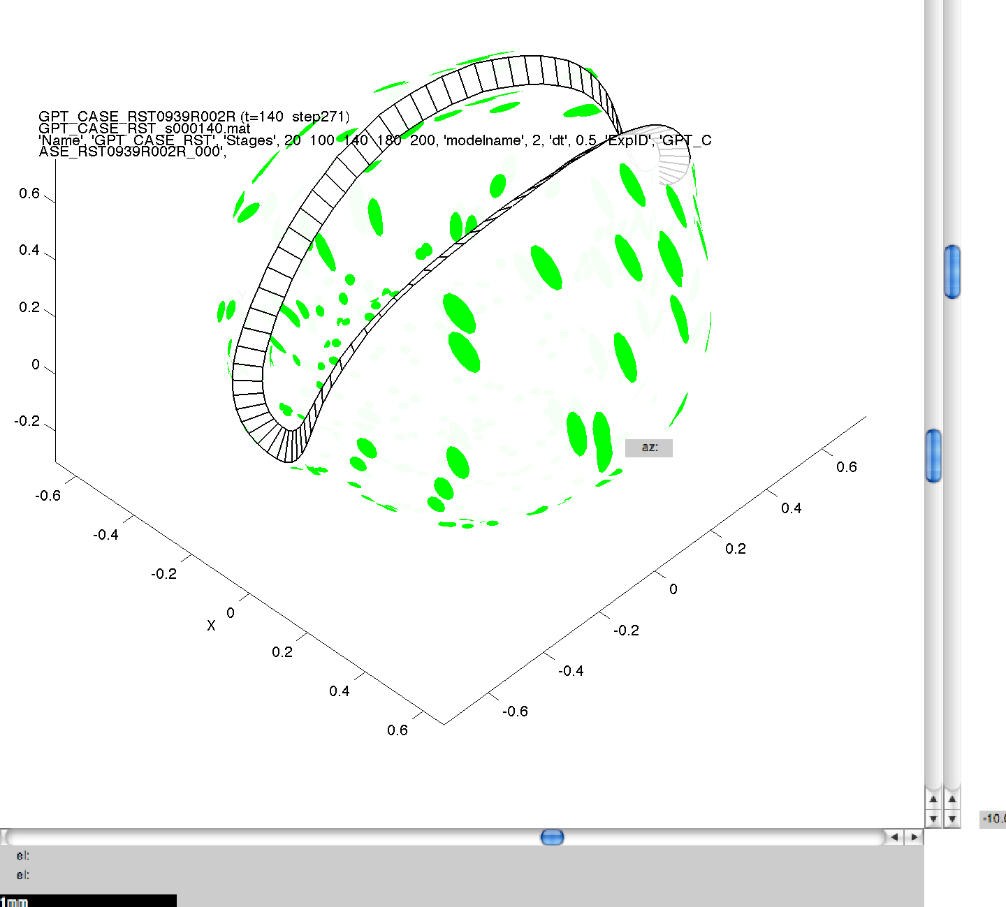
|
001GPT_CASE_RST_5 wild_.png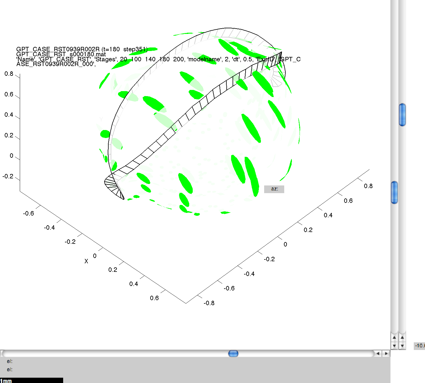
|
001GPT_CASE_RST_6 wild_.png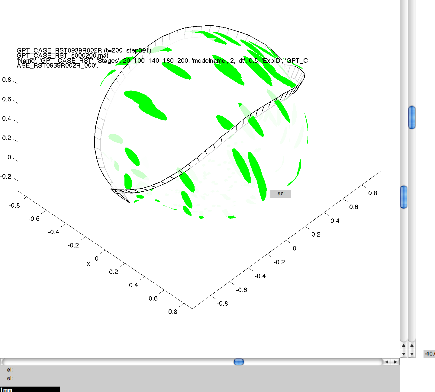
|
2) - Generating images from a simulation you ran on the cluster
NB. The results produced may not be visibly identical to those in the published literature. This is because of small, random perturbations which are applied to the initial model meshes to stop them from containing surfaces which are perfectly flat, and therefore biologically unrealistic. The results produced should be qualitatively but not quantitatively the same.
3) - Interacting with your results using the GFtbox GUI
4 Altering the simulation parameters
One such simulation parameter is dt, which is the time in seconds between iterations in the growth simulation. Large values of dt mean that fewer steps and therefore fewer calculations are required to complete a simulation. Whereas smaller values of dt mean that more steps are required, and therefore more processing time too. Therefore, a value of dt must be selected which is not so small that it is computationally unmanageable, but not so large that the observed growth is an artifact of the value of dt, rather than the underlying growth model. It is necessary therefore to test a range of values for dt to ensure that the patterns of growth observed in a simulation are consistent across the range, and to find a value which is sufficient to demonstrate the model of growth and computationally efficient.
Testing a range of dts can be achieved in several ways. One way is to use the dt argument when calling GFtboxCommand. This allows a single value to be tested. Another way is to make a batch of jobs, each using a different value for dt, by using the 'State' argument. Lastly, a range of dts can be specified in GFtboxCommand, by using the dt argument where the values within the square brackets are the dts to simulate:
       GFtboxCommand('Path','/GrowthToolbox/Models/Published/Kennaway-etal-2011/','Name','GPT_CASE_RST',...
       'Stages',[20 100 140 180 200],'modelname',3,'dt',[0.1 0.5 1 5]);
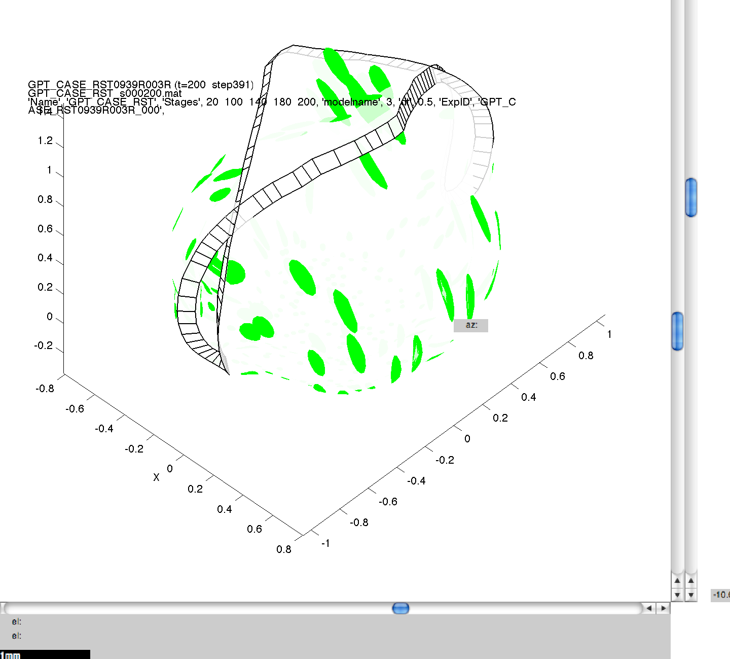
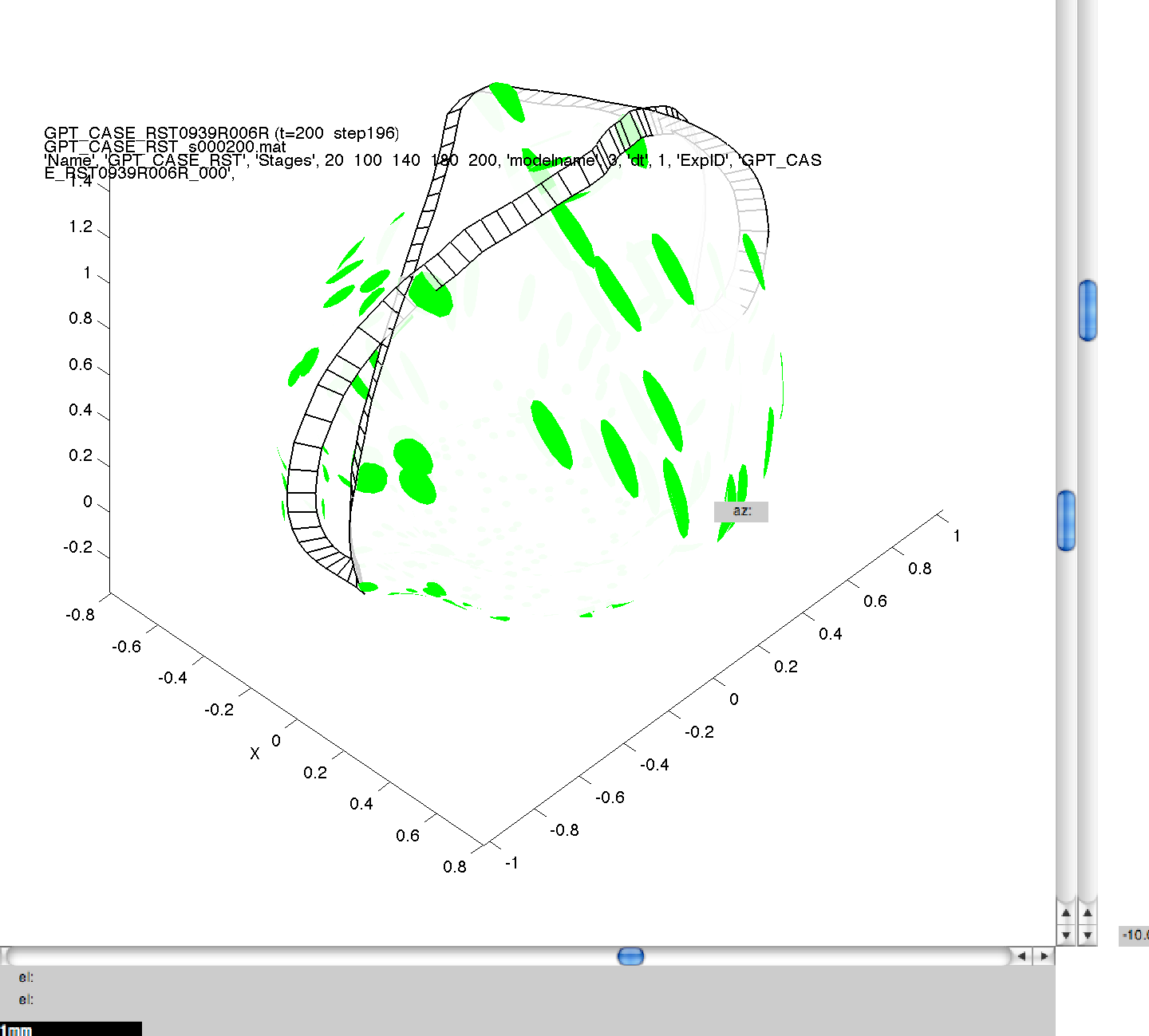
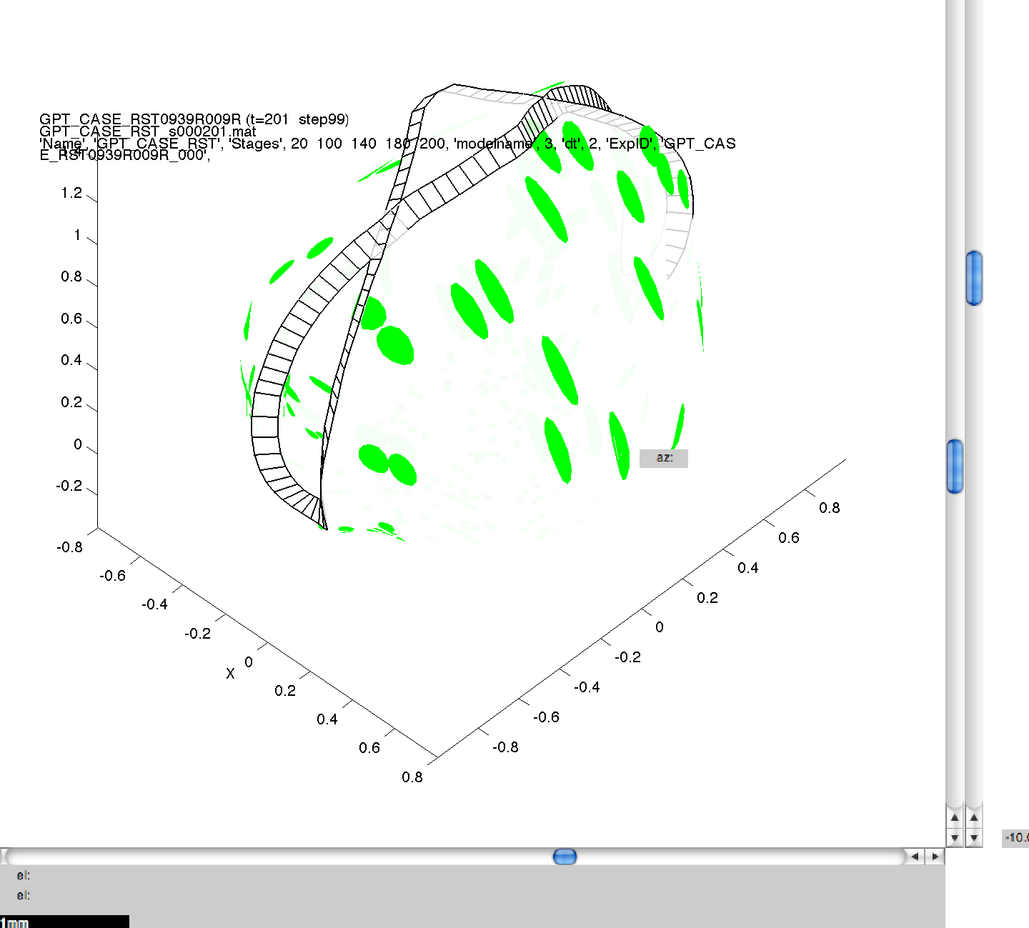
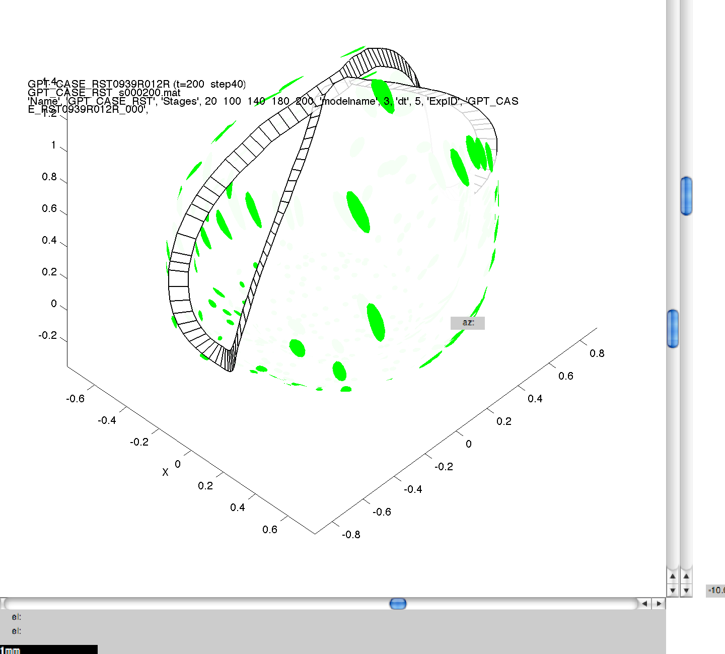
Here, we have specified four separate values for dt, and this means that four separate simulations will be run sequentially on your computer. As in 3B, images can then be generated for the mesh files produced, and compared to ensure consistency across the range of dts. In this figure, we can see the same model, at the same stage of growth, generated using the four values of dt. Though quantitatively different, they are qualitatively the same, illustrating the suitability of the default dt value of 5.
|
|
|
|
5 Altering the model parameters
It is easy to see that when even a small number of range variables, mutations or dts are specified, the total number of simulations increases quickly. If many ranges are specified, then the amount of processing time becomes unmanageable on a single computer. Via GFtboxCommand and the ClusterMonitor tool, we can remotely run a number of simulations, in parallel, on a computing cluster. It is assumed that the GrowthToolbox and Matlab are installed on your cluster, and PuTTY is required on your local computer for the tools pscp (for transferring files from your computer to a cluster) and plink (for remotely executing commands on a cluster). Using the dt range argument from 4 as an example, here we add the 'Use' name argument with the value 'Cluster':
       GFtboxCommand('State','Start','Path','/GrowthToolbox/Models/Published/Kennaway-etal-2011/','Name','GPT_CASE_RST',...
       'Stages',[20 100 140 180 200],'modelname',3,'dt',[0.1 0.5 1 5],'Use','Cluster');
The 'Cluster' option for the 'Use' name argument instructs GFtboxCommand to upload the required project directory to a remote Linux server. Instead of running the simulation on your own computer, GFtboxCommand then works out how many individual simulations are specified by the command that invoked it. In this example, the only argument which will generate multiple simulations is dt, of which there will be 4. Separate commands for each of these jobs are then automatically generated, each with an accompanying unique ID (The value of the ExpID name argument), and these are submitted as individual jobs to the cluster.
       GFtboxCommand('Name','GPT_CASE_RST','Stages',[20 100 140 180 200],'modelname',3,'dt',0.1,'ExpID','GPT_CASE_RST_1');
       GFtboxCommand('Name','GPT_CASE_RST','Stages',[20 100 140 180 200],'modelname',3,'dt',0.5,'ExpID','GPT_CASE_RST_2');
       GFtboxCommand('Name','GPT_CASE_RST','Stages',[20 100 140 180 200],'modelname',3,'dt',1,'ExpID','GPT_CASE_RST_3');
       GFtboxCommand('Name','GPT_CASE_RST','Stages',[20 100 140 180 200],'modelname',3,'dt',5,'ExpID','GPT_CASE_RST_4');
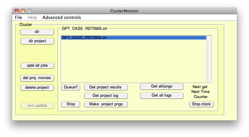
Once these jobs have been submitted, the ClusterMonitor tool opens and the new job batch ID is added to the list of jobs. Here, we will concentrate on three of the functions of ClusterMonitor: Queue?, Get project results and Make project pngs. As in part 4 of this page, these functions will enable us to visualise the growth simulation results.
| Queue Get project results Make project pngs |
|
Whilst ClusterMonitor is a useful tool for managing your cluster jobs, it is advisable to have at least a rudimentary understanding of and ability to use a Unix-based computer system. In particular, the abilities to list the contents of a folder, view the contents of a file, change the current working folder, delete, and to copy or move files or folders, are essential Unix skills for making sure everything is working as intended. It is beyond the scope of these tutorials to provide an in depth Unix tutorial (many good and simple tutorials exist on the web), but here is a short description of the Unix commands (which may be specific to our Unix-based system) that we believe to be important.
