AAMToolbox Details: Difference between revisions

From BanghamLab
Jump to navigation Jump to search
 
(7 intermediate revisions by the same user not shown)
Line 1: Line 1:
[[Software#MSERs.2C_extrema.2C_connected-set_filters_and_sieves|Back to Software]]
[[Software#Analysing_shapes_in_2D_and_3D:_AAMToolbox|Back to Software]]
==<span style="color:Navy;">What is the connection between MSER's and sieves'?</span>==
==<span style="color:Navy;">Shape modelling: what is the AAMToolbox and why'?</span>==
The papers by George Matas((Matas, et. al. 2002<ref>Matas, J., M. Urban, O. Chum and T. Pajdla (2002). ''Robust Wide baseline Stereo from Maximally Stable Extremal Regions.'' BMVC, Cardiff</ref>))((Matas et al., 2004)<ref>Matas, Jiri, et al. ''Robust wide-baseline stereo from maximally stable extremal regions''. Image and vision computing 22.10 (2004): 761-767.</ref>))
'''We wish to understand''' how biological organs grow to particular shapes. For this we need a tool to help us think through what we expect to see (''GFtbox'') and we need to make measurements of real biological organs to test our expectations (hypotheses).
(Mishkin et al., 2013)<ref>Dmytro Mishkin, Michal Perdoch,Jiri Matas (2013) ''Two-view Matching with View Synthesis Revisited'' arXiv preprint arXiv:1306.3855 </ref>  put together an effective way of finding distinguished regions (DR’s)  namely maximally stable extremal regions (<span style="color:Navy;">'''''MSER’s''''' </span>) with a powerful way of ''describing'' the regions at multiple scales and ''robustly matching'' such measurements with others in a second image. Since then many authors have confirmed the algorithms as a powerful tool for finding objects in images (review Mikolajczyk et al 2006: <ref>Krystian Mikolajczyk, Tinne Tuytelaars, Cordelia Schmid, Andrew Zisserman, Jiri Matas, Frederik Schaffalitzky, Timor Kadir, L Van Gool, (2006) ''A Comparison of Affine Region Detectors.''International Journal of Computer Vision. DOI: 10.1007/s11263-005-3848-x</ref>
<br><br>
<br><br>
<!--(This is a ''blast from the past''. I failed to popularise it at the time, however, '''MSER's are now attracting lots of attention''' so I'm now contributing my bit a little late in the day.) <br><br>-->
However, the shapes of biological organs rarely make measurement simple - how do you measure the two or three dimensional (2 or 3D) shape of an ear, leaf or Snapdragon flower? It is not enough to, for example, measure the length and width of a leaf. Why not?  
<!--[[http://cmpdartsvr3.cmp.uea.ac.uk/wiki/BanghamLab/index.php/Andrews_Organ_Recital Why the hurry?]]
#Length and width are highly correlated and so you really need only one of them
<br><br>-->
#Length and width do not capture curvature of the edges
The algorithm '''underlying''' that for finding Maximally stable extremal regions (MSER's) '''is an 'o' sieve'''. Such algorithms relate closely to mathematical morphology (dilations-erosion (Jackway et al 1996<ref>P. T. Jackway and M. Deriche. ''Scale-space properties of multiscale morphological dilation-erosion.'' IEEE Trans. Pattern Analysis and Machine Intelligence
We do it by
, 18(1):38–51</ref>) openings, closings and in particular watersheds (Vincent et al 1991 <ref>Vincent, Luc, and Pierre Soille. "Watersheds in digital spaces: an efficient algorithm based on immersion simulations." IEEE transactions on pattern analysis and machine intelligence 13.6 (1991): 583-598.</ref>) and reconstruction filters (Salembier, P. et. al. 1995<ref>Salembier P, Serra J (1995). ''Flat zones filtering, connected operators, and fi�lters by reconstruction.'' IEEE Trans Image Process 4:1153</ref>). In mathematical morphology the 'filtering' element of the MSER algorithm might be called a 'connected-set opening' ('o' sieve) . It is one of a family of closely related algorithms which for which I coined the term '''sieves'''. Why?  
*digitising the outlines using, for example, ''VolViewer''  
<br><br>
*averaging the shapes of many examples ('''Procrustes''') then find the '''principle components''' that contribute to variations from the mean shape. The different components are linearly independent of each other (not correlated). Typically most of the variation from the mean for simple leaves is captured in just the two principle components. The whole process including projections into scale space is available in the ''AAMToolbox''.
It is useful to distinguish between '''two very different signal simplifying algorithms''' both of which preserve scale-space. So called diffusion 'filters' and non-linear 'sieves'. In a filter-bank, diffusion filters (Gaussian filter) spread outliers such as impulses and sharp edged extrema over many scales whereas sieves do not (c.f. mechanical sieves in which particles either go through holes or they do not [http://en.wikipedia.org/wiki/Mesh_%28scale%29 Particle filters and sieves]). There seems to be a lot of philosophy/biology associated with arguments in favour of [http://en.wikipedia.org/wiki/Scale_space linear filters]. Why?  The non-linear 'o' sieve filter-bank appears to be a better feature finder (MSER's) and why does it have to be relevant in the natural world of biology where the fundamental signalling devices are non-linear, e.g. action potentials, GTP-binding switch proteins, etc.
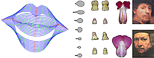
[[image:Various shapes.png|400px|center|Shape and appearance models]]Left - '''lip outlines''' vary along the first principle component. Next - '''leaf and petal''' shapes. Right - Rembrandt's '''self portraits''' vary.
|}
 
====<span style="color:Navy;">What do we know about sieves?</span>====
As low-pass filters sieves robustly reject outliers (Bangham, J.A. 1993<ref>Bangham, JA (1993) ''Properties of a Series of Nested Median Filters, Namely the Data Sieve.'' IEEE Transactions on Signal Processing, 41 (1). pp. 31-42. ISSN 1053-587X</ref>). Whilst it is clear that by 'knocking off' outliers they cannot introduce new extrema we formally proved that by this definition they preserve '''''scale-scale space''''' (Bangham et al 1996<ref>Bangham, JA, Harvey, RW, Ling, PD and Aldridge, RV (1996) ''Morphological scale-space preserving transforms in many dimensions.'' The Journal of Electronic Imaging (JEI), 5 (3). pp. 283-299.</ref>Bangham et al 1996b<ref>Bangham, JA, Chardaire, P, Pye, CJ and Ling, PD (1996) ''Multiscale nonlinear decomposition: The sieve decomposition theorem.'' IEEE Transactions on Pattern Analysis and Machine Intelligence, 18 (5). pp. 529-539. ISSN 0162-8828</ref> (c.f. the properties of multiscale dilation and erosion (Jackway et al 1996<ref>Jackway, P.T. and Deriche, M. (1996) ''Scale-space properties of the multiscale morphological dilation-erosion'' IEEE Transactions on Pattern Analysis and Machine Intelligence, vol.18, no.1, pp.38,51</ref> )<br><br>
'''Applications''' in addition to their role in MSERs. Whilst 2D MSER's (sieves in our old terminology) are used for finding objects in 2D image we have also used sieves in other ways, indeed we started in 1D. For example analysing protein hydrophobicity plots(Bangham, 1988<ref>Bangham, J.A. (1988). ''Data-sieving hydrophobicity plots. Anal. Biochem''. 174, 142–145</ref>), de-noising single channel current data(Bangham et al, 1984<ref>Bangham, J.A., and T.J.C. Jacob (1984). ''Channel Recognition Using an Online Hardware Filter''. In Journal of Physiology, (London: Physiological Society), pp. 3–5</ref>), texture analysis(Southam et al, 2009<ref>Southam, P., and Harvey, R. (2009). ''Texture classification via morphological scale-space: Tex-Mex features''. J. Electron. Imaging 18, 043007–043007</ref>), lipreading(Matthews et al., 2002<ref>Matthews, I., Cootes, T.F., Bangham, J.A., Cox, S., and Harvey, R. (2002). ''Extraction of visual features for lipreading''. Pattern Anal. Mach. Intell. Ieee Trans. 24, 198–213</ref>). In 2D for segmenting 2D through extremal trees(Bangham et al., 1998<ref>Bangham, J.A., Hidalgo, J.R., Harvey, R., and Cawley, G. (1998). ''The segmentation of images via scale-space trees''. In Proceedings of British Machine Vision Conference, pp. 33–43</ref>), maximally stable contours(Lan et al., 2010<ref>Lan, Y., Harvey, R., and Perez Torres, J.R. (2010). ''Finding stable salient contours.'' Image Vis. Comput. 28, 1244–1254</ref>), images (), creating painterly pictures from photos(Bangham et al., 2003<ref>Bangham, J.A., Gibson, S.E., and Harvey, R. (2003). T''he art of scale-space''. In Proc. British Machine Vision Conference, pp. 569–578</ref>); and in 3D for segmenting volumes.
 
==References==
<references />
 
==<span style="color:Navy;">How does this measure shapes?</span>==
==<span style="color:Navy;">Limitations?</span>==

Latest revision as of 15:08, 28 November 2013

Back to Software

Shape modelling: what is the AAMToolbox and why'?

We wish to understand how biological organs grow to particular shapes. For this we need a tool to help us think through what we expect to see (GFtbox) and we need to make measurements of real biological organs to test our expectations (hypotheses).

However, the shapes of biological organs rarely make measurement simple - how do you measure the two or three dimensional (2 or 3D) shape of an ear, leaf or Snapdragon flower? It is not enough to, for example, measure the length and width of a leaf. Why not?

  1. Length and width are highly correlated and so you really need only one of them
  2. Length and width do not capture curvature of the edges

We do it by

  • digitising the outlines using, for example, VolViewer
  • averaging the shapes of many examples (Procrustes) then find the principle components that contribute to variations from the mean shape. The different components are linearly independent of each other (not correlated). Typically most of the variation from the mean for simple leaves is captured in just the two principle components. The whole process including projections into scale space is available in the AAMToolbox.
Shape and appearance models

Left - lip outlines vary along the first principle component. Next - leaf and petal shapes. Right - Rembrandt's self portraits vary.