AAMToolbox viewing one population in shape space: Difference between revisions
Jump to navigation
Jump to search
(Created page with 'Back to Tutorial pages<br> =<span style="color:Navy;">'''What''' is Shape Space?</span>= <br><br> ===<span style="color:FireBrick;…') |
No edit summary |
||
| Line 6: | Line 6: | ||
{| border="0" cellpadding="5" cellspacing="3" | {| border="0" cellpadding="5" cellspacing="3" | ||
|- valign="top" | |- valign="top" | ||
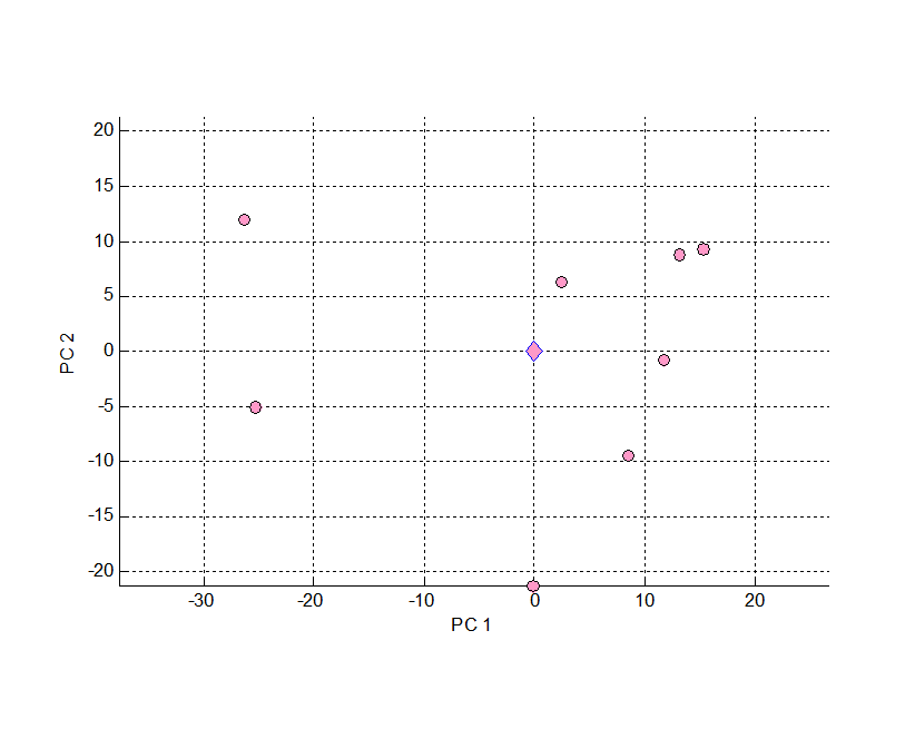
|width="400pt"|The pink diamond shows the position of the mean cartoon shape plotted in shape space.<br><br> | |width="400pt"|The''' pink diamond''' shows the position of the '''mean''' cartoon shape plotted in shape space.<br><br> | ||
Each spot represents one of the input point models (images).<br><br> | Each '''spot''' represents one of the''' input point models''' (images).<br><br> | ||
Each point model represents 38 points i.e. 38*2=76 values in the normal two dimensional viewing space OR a single point in 72 dimensional space. However, we cannot visualise 78 dimensional space so we have used PCA to choose a view point (a rotation of the space) such that we can see the two principle components. | Each point model represents 38 points i.e. 38*2=76 values in the normal two dimensional viewing space OR a single point in 72 dimensional space. However, we cannot visualise 78 dimensional space so we have used PCA to choose a view point (a rotation of the space) such that we can see the two principle components. This allows us to visualise and '''focus on the significant (in the sense of accounting for the most variance) parameters'''. Of course, it might be another component that is most significant in biological terms. It is also quite possible that the biologically important parameters are correlated non-linearly in which case they could be invisible in this project because they are distributed into the new components as awkwardly as they were in the original data. | ||
|width="400pt"|[[File:Cartoons_shape_space_1_AAMToolbox.png|400px|Shape space]]<br>Shape Space: the principle component is plotted on the x-axis (abscissa) and the component that accounts for the second largest amount of variation is plotted on the y-axis (ordinate). Pink diamond shows the position of the mean shape. The other points | |width="400pt"|[[File:Cartoons_shape_space_1_AAMToolbox.png|400px|Shape space]]<br>Shape Space: the principle component is plotted on the x-axis (abscissa) and the component that accounts for the second largest amount of variation is plotted on the y-axis (ordinate). Pink diamond shows the position of the mean shape. The other points | ||
|} | |} | ||
| Line 14: | Line 14: | ||
{| border="0" cellpadding="5" cellspacing="3" | {| border="0" cellpadding="5" cellspacing="3" | ||
|- valign="top" | |- valign="top" | ||
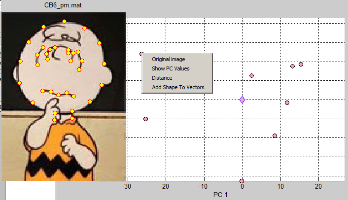
|width=" | |width="150pt"|Each''' pink circle marker represents a data sample'''. Right clicking on a marker opens a context menu. Here we have selected to view the associated original image and its point model (shown to the left). <br><br> | ||
Showing the PC values causes them to be echoed to the command window.<br><br> | Showing the PC values causes them to be echoed to the command window.<br><br> | ||
|width="600pt"|[[File:Cartoons_shape_space_2_AAMToolbox.png|600px|Shape space]]<br>Shape Space context menu for the markers. The top-left sample has been selected and the associated image/point model is shown on the left. | |||
|width=" | |} | ||
{| border="0" cellpadding="5" cellspacing="3" | |||
|- valign="top" | |||
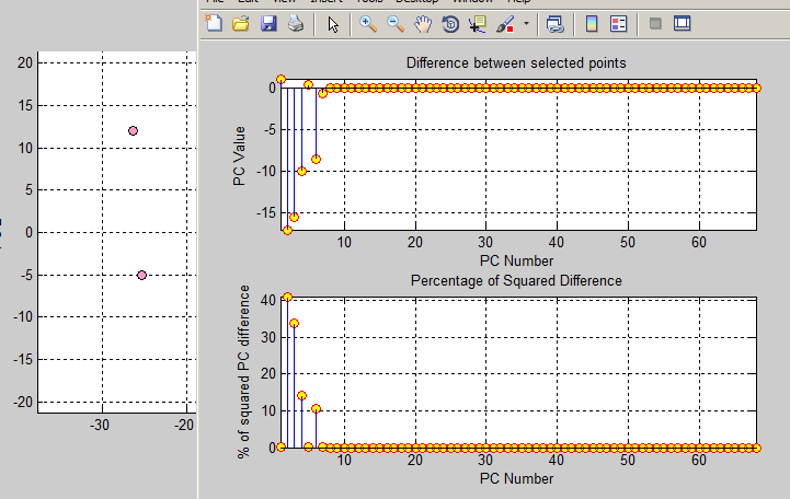
|width="150pt"|Right clicking on a marker opens a context menu. Here we have selected to view the distance between the two visible markers. The distances (and squared distances) for each of the components is shown in the right. <br><br> | |||
Showing the PC values causes them to be echoed to the command window.<br><br> | |||
|width="600pt"|[[File:Cartoons_shape_space_3_AAMToolbox.png|600px|Shape space]]<br>Shape Space: distance between two points. | |||
|} | |} | ||
Revision as of 11:00, 21 February 2012
What is Shape Space?


