AAMToolbox viewing statistical model: Difference between revisions

From BanghamLab
Jump to navigation Jump to search
(Created page with 'Back to Tutorial pages<br> =<span style="color:Navy;">Viewing shape and appearance models in 2D</span>= ==Principle component analy…')
 
No edit summary
 
(5 intermediate revisions by the same user not shown)
Line 1: Line 1:
[[Tutorials on the Shape modelling toolbox#1|Back to Tutorial pages]]<br>
[[Tutorials on the Shape modelling toolbox#1|Back to Tutorial pages]]<br>
=<span style="color:Navy;">Viewing shape and appearance models in 2D</span>=
==Principle component analysis of point-models and image pixel values (appearance models)==
 
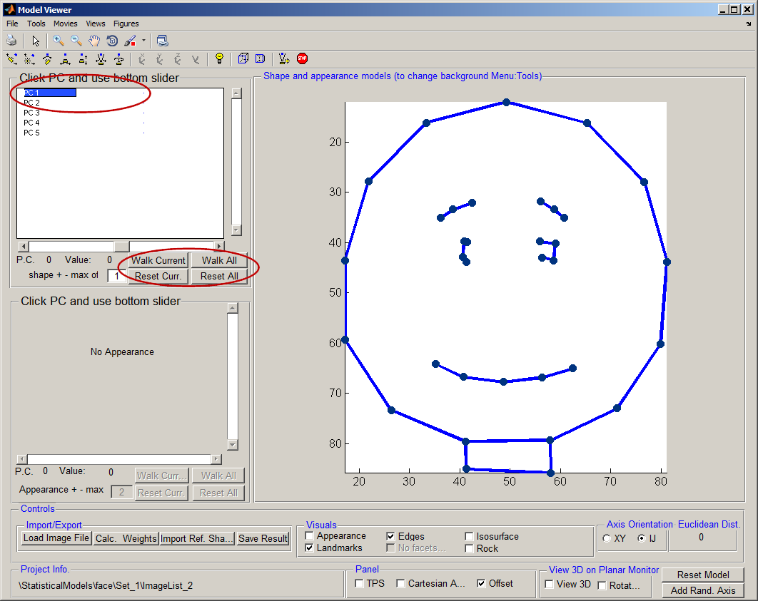
To view results from the PCA select '''View Stats Model'' from the AAMToolbox control panel: <br><br>
=<span style="color:Navy;">Walking through contributions of principle components.</span>=
=<span style="color:Navy;">View shape models</span>=
<br><br>
*Shape model
[[File:Walk_model_AAMToolbox.png|700px|Model Viewer]]<br><br>
**Input: landmark points, i.e. the point-models for all images of interest.
===<span style="color:FireBrick;">Mean shape</span>===
**Output: mean shape and associated shape model that captures deviations from the mean. Enough principle components are included to account for 95% of the variance from the mean (set using Options).
{| border="0" cellpadding="5" cellspacing="3"
*Appearance model
|- valign="top"
**Input: landmark points, i.e. the point-models together with the image intensity within triangles determined by a Delauny triangulation of the points.
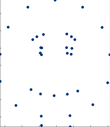
|width="700pt"|The dots on the right represent the mean positions of the landmarks averaged over all the images in the model. These points mean more to us once they are joined by lines (see above screenshot). Capturing that higher meaning requires more analysis or, as in this case, human interaction (when we created the template).<br><br>Note that the point models had been normalised to the''' same scale, same rotation and same translational''' position.<br>
**Output: mean appearance and associated appearance model that captures deviations from the mean.  
|width="200pt"|[[File:Mean_shape.png|200px|The Model generator control panel]]
=<span style="color:Navy;">Statistical Model Generator control panel.</span>=
|}
Showing the steps (in red) to build a statistical model.<br>
===<span style="color:FireBrick;">Variations along the principle component axis</span>===
Notice: the set of landmarks represented as stars will be included in the shape model, in this case all of them. For this model you can accept the default settings and jump directly to step 3 and select all the images. Then compute the principle component analysis (PCA) using step 4 and return to the AAMToolbox on the way to viewing the results.<br><br>
{| border="0" cellpadding="5" cellspacing="3"
[[File:Model_generator_AAMToolbox.png|822px|The Model generator control panel]]<br><br>
|- valign="top"
==Steps to build a shape model using principle component analysis (PCA)==
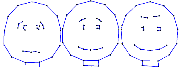
|width="700pt"|To visualise sliding (walking) along an axis imagine a straight line fitted to a set of data points. Then read-out the x,y coordinates as we move back and forth along the line. Correlation between x and y (the straight line) means that the outputs are correlated. In this model we are doing a similar thing as we slide along the axis (fitted line) we read-out values in the model coordinate system that are then transformed (by the model) back into the viewing coordinates. <br><br>[[File:PC1_cartoon_combined.png|200px|The Model generator control panel]]<br> Left, minus one standard deviation along PC1.<br>Middle, mean shape. <br>Right, plus one standard deviation along PC1.
===<span style="color:FireBrick;">Step 1) Options</span>===
|width="300pt"|<wikiflv width="300" height="300" logo="false"  loop="true" background="white">CartoonPC1.flv|CartoonPC1.png</wikiflv><br>Sliding (walking) along the principle component axis.
[[File:Stats_Model_Options_AAMToolbox.png|500px|The Model generator control panel]]<br><br>
|}
*The first step in PCA is to align all the point models. In this case we assume that the images should be normalised to the''' same scale, same rotation and same translational''' position. This might not always be the case. If we want to model leaf growth then the point model should '''not''' be scaled. Alternatively, if we want to capture the pose of a face portrait the point models should not be rotationally aligned.<br>
===<span style="color:FireBrick;">Variations along axis with the next largest variation</span>===
For the '''cartoon faces we normalise for all three'''.
{| border="0" cellpadding="5" cellspacing="3"
|- valign="top"
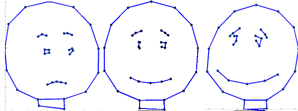
|width="700pt"|<br><br>[[File:PC1_cartoon_combined2.png|200px|+1 and -1 standard deviation from the mean]]<br> Left, minus one standard deviation along PC2.<br>Middle, mean shape. <br>Right, plus one standard deviation along PC2.
|width="300pt"|<wikiflv width="300" height="300" logo="false"  loop="true" background="white">CartoonPC2.flv|CartoonPC2.png</wikiflv><br>Sliding (walking) along the axis accounting for the second most amount of variation.
|}

Latest revision as of 11:24, 9 March 2012

Back to Tutorial pages

Viewing shape and appearance models in 2D

Walking through contributions of principle components.


Model Viewer

Mean shape

The dots on the right represent the mean positions of the landmarks averaged over all the images in the model. These points mean more to us once they are joined by lines (see above screenshot). Capturing that higher meaning requires more analysis or, as in this case, human interaction (when we created the template).

Note that the point models had been normalised to the same scale, same rotation and same translational position.
The Model generator control panel

Variations along the principle component axis

To visualise sliding (walking) along an axis imagine a straight line fitted to a set of data points. Then read-out the x,y coordinates as we move back and forth along the line. Correlation between x and y (the straight line) means that the outputs are correlated. In this model we are doing a similar thing as we slide along the axis (fitted line) we read-out values in the model coordinate system that are then transformed (by the model) back into the viewing coordinates.

The Model generator control panel
Left, minus one standard deviation along PC1.
Middle, mean shape.
Right, plus one standard deviation along PC1.
<wikiflv width="300" height="300" logo="false" loop="true" background="white">CartoonPC1.flv|CartoonPC1.png</wikiflv>
Sliding (walking) along the principle component axis.

Variations along axis with the next largest variation


+1 and -1 standard deviation from the mean
Left, minus one standard deviation along PC2.
Middle, mean shape.
Right, plus one standard deviation along PC2.
<wikiflv width="300" height="300" logo="false" loop="true" background="white">CartoonPC2.flv|CartoonPC2.png</wikiflv>
Sliding (walking) along the axis accounting for the second most amount of variation.