MSER and Sieve Details

Back to Software

What is the connection between MSER's and sieves'?

The papers by George Matas((Matas, et. al. 2002<ref>Matas, J., M. Urban, O. Chum and T. Pajdla (2002). Robust Wide baseline Stereo from Maximally Stable Extremal Regions. BMVC, Cardiff</ref>))((Matas et al., 2004)<ref>Matas, Jiri, et al. Robust wide-baseline stereo from maximally stable extremal regions. Image and vision computing 22.10 (2004): 761-767.</ref>)) (Mishkin et al., 2013)<ref>Dmytro Mishkin, Michal Perdoch,Jiri Matas (2013) Two-view Matching with View Synthesis Revisited arXiv preprint arXiv:1306.3855 </ref> put together an effective way of finding distinguished regions (DR’s) namely maximally stable extremal regions (MSER’s ) with a powerful way of describing the regions at multiple scales and robustly matching such measurements with others in a second image. Since then many authors have confirmed the algorithms as a powerful tool for finding objects in images (review Mikolajczyk et al 2006: <ref>Krystian Mikolajczyk, Tinne Tuytelaars, Cordelia Schmid, Andrew Zisserman, Jiri Matas, Frederik Schaffalitzky, Timor Kadir, L Van Gool, (2006) A Comparison of Affine Region Detectors.International Journal of Computer Vision. DOI: 10.1007/s11263-005-3848-x</ref>, Kimmel 2011 <ref>Kimmel, R., Zhang, C., Bronstein, A.M., Bronstein, M. (2011) Are MSER features really interesting? IEEE Trans. Pattern Analysis and Machine Intelligence 33:2316–2320</ref>

The algorithm underlying that for finding Maximally stable extremal regions (MSER's) is an 'o' sieve. Such algorithms relate closely to mathematical morphology (dilations-erosion (Jackway et al 1996<ref>P. T. Jackway and M. Deriche. Scale-space properties of multiscale morphological dilation-erosion. IEEE Trans. Pattern Analysis and Machine Intelligence , 18(1):38–51</ref>) openings, closings and in particular watersheds (Vincent et al 1991 <ref>Vincent, Luc, and Pierre Soille. "Watersheds in digital spaces: an efficient algorithm based on immersion simulations." IEEE transactions on pattern analysis and machine intelligence 13.6 (1991): 583-598.</ref>) and reconstruction filters (Salembier, P. et. al. 1995<ref>Salembier P, Serra J (1995). Flat zones filtering, connected operators, and filters by reconstruction. IEEE Trans Image Process 4:1153</ref>). In mathematical morphology the 'filtering' element of the MSER algorithm might be called a 'connected-set opening' ('o' sieve) . It is one of a family of closely related algorithms which for which I coined the term sieves. Why?

Why call the family of feature finding algorithms sieves and not filters?

I thought it may be helpful to distinguish between two very different signal simplifying algorithms both of which preserve scale-space: linear 'filters' and non-linear 'sieves'. In a linear-filter-bank such as a bank of Gaussian filters the input signal is separated, prism like, into frequency related scale bands (large and small blobs). Like all linear filters they spread outliers such as impulses and sharp edges over many scales. Despite these disadvantages Gaussian filters have nearly an overwhelmingly useful property namely ...

Gaussian filters preserve scale space

In the 1980's-1990's there were many publications on the properties of Gaussian (diffusion) filters. Key is that they preserve scale-space (Babaud et. al. 1986 "The uniqueness of the Gaussian kernel ...")<ref>Babaud, Jean; Witkin, Andrew P.; Baudin, Michel; Duda, Richard O., "Uniqueness of the Gaussian Kernel for Scale-Space Filtering," Pattern Analysis and Machine Intelligence, IEEE Transactions on , vol.PAMI-8, no.1, pp.26,33, Jan. 1986 doi: 10.1109/TPAMI.1986.4767749</ref> To understand what is meant: imagine a photo projected onto a wall using a data projector. Leave it on for an hour. Then turn of the projector. Regions that were illuminated (white) will be warmer than those that were black. Now turn the projector off and turn on an infrared image viewer. Once again the image will be visible (warm and cold regions showing up). However, as we wait heat will diffuse from the warm to cooler regions - the image will become blurred. Heat will never flow to form new extrema. If the thermal conductivity of the surface is uniform and anisotropic then there is one simple filter that will produce the same result. A Gaussian blur filter.

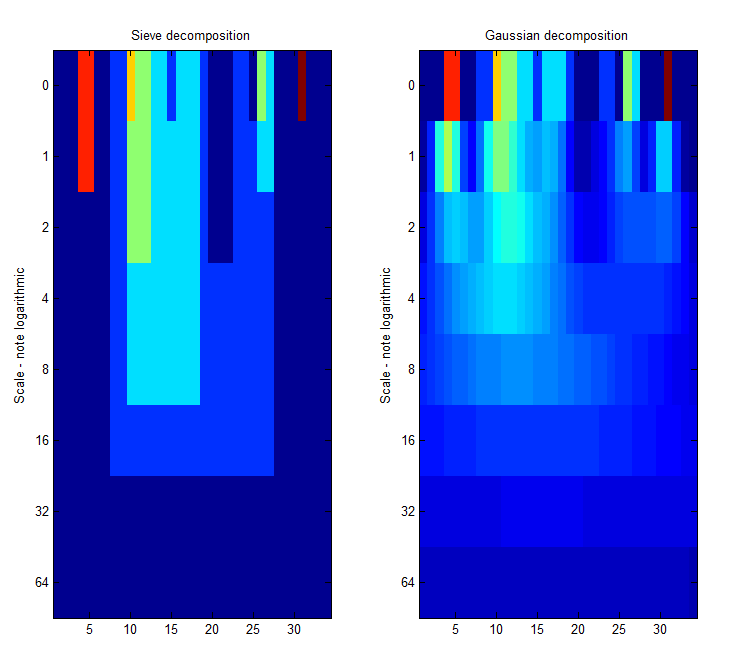
Here, we have three panels illustrating one dimensional signals represented in scale space. I have used 'heat maps' to represent the signal intensity at each scale.

Consider a signal, <math>X</math> X=getData('PULSES3WIDE') >blue X=0 5 5 0 0 1 1 4 3 3 2 2 1 2 2 2 1 0 0 0 1 1 0 3 2 0 0 0 6 0 0

The data has minima and maxima of different scales (lengths).

Left Panel. Here, a A low-pass siv4.m gradually removes extrema (from the signal shown above) as scale increases from scale 1 to scale 64. The resulting traces are shown as a 'heat map' where the signal goes from left to right, bright colours like red are large amplitude, small scale extrema. At each increasing scale (down the map) extrema have been removed. The 'm'-sieve preserves scale-space so no new extrema (light regions) are formed as we move to increasing scales. Moreover, the features do not wander about in scale-space. We could say that in one dimension we measure pulse length using a sieve just as we might use a ruler or measuring tape in the physical world.
Middle Panel. A Gaussian filter bank also preserves scale-space as shown by Witkin 1986. No new features (local extrema) are formed. However, the features wander about in scale-space.
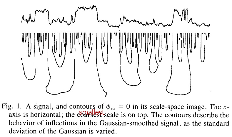
(Babaud et. al. 1986 "The uniqueness of the Gaussian kernel ...")<ref>Babaud, Jean; Witkin, Andrew P.; Baudin, Michel; Duda, Richard O., "Uniqueness of the Gaussian Kernel for Scale-Space Filtering," Pattern Analysis and Machine Intelligence, IEEE Transactions on , vol.PAMI-8, no.1, pp.26,33, Jan. 1986 doi: 10.1109/TPAMI.1986.4767749</ref>
Right Panel, Babaud's original Figure showing heat-map 'isotherms'. (Actually, to be consistent with the other Panels I have flipped the image vertically.) The features wander about in scale-space and sharp edged features do not sharply disappear - they are smudged over scale-space.

• Small, hot areas (outliers) are smoothed out as are sharp edges.
• Sieves are the opposite, impulses and regions with sharp edges do not spread over many scales

(c.f. mechanical sieves in which particles (granules) either go through holes or they do not Particle filters and sieves.) They do however, spread smooth waveforms over many scales. Gaussian filter banks and filter banks based on sieves are complementary to each other.

Superficially it is clear that, by 'knocking off' outliers at increasingly large scales, sieves cannot introduce new extrema but to clarify the issue we formally proved that they do not introduce new extrema, i.e. preserve scale-space (Bangham et al 1996<ref>Bangham, JA, Harvey, RW, Ling, PD and Aldridge, RV (1996) Morphological scale-space preserving transforms in many dimensions. The Journal of Electronic Imaging (JEI), 5 (3). pp. 283-299.</ref>Bangham et al 1996b<ref>Bangham, JA, Chardaire, P, Pye, CJ and Ling, PD (1996) Multiscale nonlinear decomposition: The sieve decomposition theorem. IEEE Transactions on Pattern Analysis and Machine Intelligence, 18 (5). pp. 529-539. ISSN 0162-8828</ref>, c.f. the properties of multiscale dilation and erosion, Jackway et al 1996<ref>Jackway, P.T. and Deriche, M. (1996) Scale-space properties of the multiscale morphological dilation-erosion IEEE Transactions on Pattern Analysis and Machine Intelligence, vol.18, no.1, pp.38,51</ref>). Preserving scale-space is one of the important reasons why MSER's are so useful for finding interesting regions worth further characterisation.

Implementation

One dimensional sieves are easily implemented by run-length coding the signal, each extremum has a list of just two neighbours. Indeed, in collaboration with CCL we implemented the algorithm on a PC board to characterise the output, in real time, from line-scan cameras (often used industrially when, in the early 1990's, 2D digital camera's were not easily available). Implementations for images in higher dimensions are similar but keeping track of lists of neighbours is a little more complex, but see Nister and Stewenius, <ref>D. Nister and H. Stewenius Linear time maximally stable extremal regions ECCV 2008 part II LNCS 5303 pp 183-196. </ref> for a cool implementation of the MSER algorithm.

Applications

In addition to their role finding in objects in 2D images we have used sieves to analyse 1, 2 and 3D signals. We started in 1D (digital images were not available at the time). For example analysing protein hydrophobicity plots(Bangham, 1988<ref>Bangham, J.A. (1988) Data-sieving hydrophobicity plots. Anal. Biochem. 174, 142–145</ref>) for which it was found by Fasman (1990) <ref>Fasman and Gilbert "The prediction of transmembrane protein sequences and their conformation: an evaluation" in Trends in Biochemistry 15 pp 89:91</ref> to "correctly predict the hydrophobic transmembrane regions ..." (see more details). , de-noising single channel current data (Bangham et al, 1984<ref>Bangham, J.A., and T.J.C. Jacob (1984). Channel Recognition Using an Online Hardware Filter in The Journal of Physiology, (London: Physiological Society), pp. 3–5</ref>). Much later we used them for texture analysis (Southam et al, 2009<ref>Southam, P., and Harvey, R. (2009). Texture classification via morphological scale-space: Tex-Mex features. J. Electron. Imaging 18, 043007–043007</ref>) and lipreading (Matthews et al., 2002<ref>Matthews, I., Cootes, T.F., Bangham, J.A., Cox, S., and Harvey, R. (2002). Extraction of visual features for lipreading. Pattern Anal. Mach. Intell. Ieee Trans. 24, 198–213</ref>). In 2D for segmenting images through extremal trees (c.f. MSER's) (Bangham et al., 1998<ref>Bangham, J.A., Hidalgo, J.R., Harvey, R., and Cawley, G. (1998). The segmentation of images via scale-space trees. In Proceedings of British Machine Vision Conference, pp. 33–43</ref>), maximally stable contours(Lan et al., 2010<ref> Lan, Y., Harvey, R., and Perez Torres, J.R. (2010). Finding stable salient contours. Image Vis. Comput. 28, 1244–1254</ref>), creating painterly pictures from photos (Bangham et al., 2003<ref>Bangham, J.A., Gibson, S.E., and Harvey, R. (2003). The art of scale-space. In Proc. British Machine Vision Conference, pp. 569–578</ref>)(Fo2Pix sold about 65,000 licences for our software package: ArtMaster); and in 3D for segmenting volumes in CAT scans.

Could non-linear filter banks (sieves) have evolved in biological systems?

Biological systems are too complex too huge to comprehend without some initial insights. In vision the particular theoretical 'torches' that light the experimental findings are the Fourier transform, Gaussian or Gabor filter banks. We look where those lights are shining and what we find seems to fits that intuition e.g. Gaussian/Gabor. Or perhaps has to fit for want of other torches'.

So care is needed. Science should be creative, we should create a number of torches pointing in different directions (based on different theoretical frameworks where possible) then use experimental evidence to reject those that do not fit leaving us with the best hypothesis, theoretical framework, so far.

We now know that sieves (MSER's) not only exist but offer significant practical advantages over other methods in computer vision. They are an alternative 'torch' that might need rejecting. Perhaps we should re-evaluate the biological evidence. Could the brain be understood in terms of sieves? Were this to be the case then it could change what we look for brain structures. Hardware implementations of sieves are all about connectivity and relative thresholds as are brains, so perhaps it is possible.

• our hardware implementation of the 1D filter bank was very different to a linear filter bank.
• Likewise the linear time implementation of the 2D MSER algorithm (Nister and Stewenius, <ref>D. Nister and H. Stewenius Linear time maximally stable extremal regions ECCV 2008 part II LNCS 5303 pp 183-196. </ref>) in which dynamic connectivity is everything.
  
  

Exploring this problem would be just the 'wild' opportunity that I have enjoyed exploring in my research life. It would be a wild ride whatever the outcome - unfortunately cancer now (June 2014) leaves me out of the game..

Summary of basic properties of sieves, linear and non-linear filters?

	Sieve 1D	Sieve 2D	Sieve 3D	Gaussian 1D	Gaussian 2D	Median 1D	Median 2D
Preserve Scale space	Yes	Yes	Yes	Yes	Yes	No	No
Separate signals by	Length	Area	Volume	Pulse Frequency	Blob Frequency 2D	Roughly Pulse length	Roughly Blob Area

References

<references />