One dimensional sieve applied to images

Return to MSERs and extrema

'siv4.mex' implemenation applies the m-sieve column wise

A Matlab function siv4_test.m illustrates how siv4.mex can be used to analyse columns of 1D data.

Consider a signal, <math>X</math> X=getData('PULSES3WIDE') >blue X=0 5 5 0 0 1 1 4 3 3 2 2 1 2 2 2 1 0 0 0 1 1 0 3 2 0 0 0 6 0 0

The data has minima and maxima of different scales (lengths). In one dimension we measure pulse length using a ruler, measuring tape or whatever - but not frequency or Gaussian scale.

Filter

Lowpass siv4.mex

Imagine that within the data above there is a signal, which may comprise positive or negative pulses, that is contaminated by smaller scale noise (leftmost panel). 'siv4.mex' (i.e. compiled from the 'C' to suite your operating system) can filter out the smaller scale noise - irrespective of amplitude. The rightmost panels show the results of removing all 'noise' less than scales 1, 5 and 10. Unlike linear filters edges remain well defined and 'noise' is completely removed.

data{1}=siv4_alt('PULSES3WIDE',[2;5;10]);
data{1}
       ans = 
         y: {[34x1 double]  [34x1 double]  [34x1 double]} % outputs for the 3 specified scales
      scan: [34 34]            % instructing single column processing
         X: [34x1 double]    % input data
   options: [3x4 double]   % options (see elsewhere)
   outputs: 'lll'                 % outputs all lowpass
      type: 'int'                 % input data may be double but only contains integers
      name: 'PULSES3WIDE'

Non-linear: the starting point for MSER's

A low-pass 'o' sieve scale 1 (non-linear filter underpinning the MSER algorithm) can remove scale 1 maxima. The result is shown in red, extrema at <math>M^1_8</math> , <math>M^1_{24}</math> , <math>M^1_{29}</math> have been removed. There is no blur. The remaining signal is unchanged.

scaleA=1;
Y1=SIVND_m(X,scaleA,'o');

Scale 2 maxima are removed next using the 'o' sieve scale 2. The result is shown in green. Extrema at <math>M^2_{14}</math> , <math>M^2_{21}</math> have been removed. Still no blur and what remains is unchanged.

scaleB=2;
Y2=SIVND_m(X,scaleB,'o');

A high-pass 'o' sieve scale 1 shows the extrema that have been removed. In red the scale 1 extrema at <math>M^1_8</math> , <math>M^1_{24}</math> , <math>M^1_{29}</math> have been removed. In green extrema of scale 2 are shown. In the sieve terminology these are granules. Think of grading gravel using sieves, large holes let through large grains and small holes let through small grains. Here scale is measured as length. If granules don't fit they don't get through - unlike linear filters which leak.

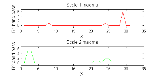
red=double(X)-double(Y1); 
green=double(Y1)-double(Y2);

Repeat over scales 0 to 15

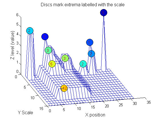
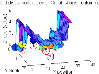
Increasing the scale (towards the front) removes extrema of increasing length. The algorithm cannot create new maxima (it is an 'o' sieve) it is, therefore, scale-space preserving.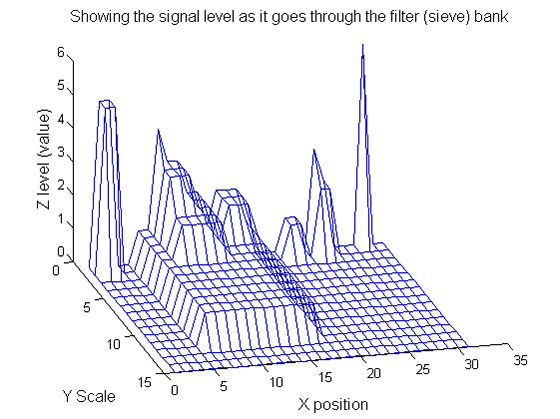

YY=ones([length(X),1+maxscale]);
for scale=0:maxscale
    Y2=SIVND_m(Y1,scale,'o',1,'l',4);
    YY(:,scale+1)=Y2';
    Y1=Y2; % each stage of the filter (sieve) is idempotent
end

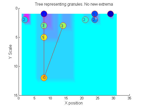
Label the granules

We can create a data structure that captures the properties of each granule. The number in each disc indicates the granule scale. Each cell in the PictureElement field has a list of indexes recording the granule position (<math>X</math>). (In 1D this is best done run-length coded but this code is designed to also work in 2D.)

g=SIVND_m(X,maxscale,'o',1,'g',4);
g =   Number: 10
             area: [1 1 1 2 2 2 3 3 5 12]
            value: [6 1 1 2 5 1 1 1 1 1]
            level: [6 4 3 2 5 1 3 2 2 1]
        deltaArea: [5 2 1 7 3 12 2 2 7 19]
        last_area: [6 3 2 9 5 14 5 5 12 31]
             root: [29 8 24 24 2 21 8 14 8 8]
   PictureElement: {1x10 cell}

g.PictureElement

 Columns 1 through 9

   [29]    [8]    [24]    [2x1 double]    [2x1 double]    [2x1 double]    [3x1 double]    [3x1 double]    [5x1 double]  [12x1 double]

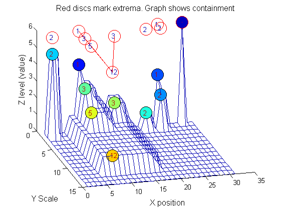
Tracing the granules through scale-space identifies candidate MSER's

The granules contain all the information in the signal. The tree illustrates the relationship between granules. The granules at <math>X=8</math> (scales 1, 3, 5, 12) indicates a region that is stable over scale. Likewise at <math>X=24</math> (scales 1, 2). One might argue that the latter is the less stable.

We have candidate 1D MSER's

Which is the most stable?

This is a pragmatic judgement. Parameters might include

1. how stable over scale (length)
2. amplitude (value or level)
3. a vector of amplitude over scale
4. proximity to others

So far maxima. What about minima and more?

The filter (sieve) that finds maxima is a connect-set opening ('o' sieve). A 'c' sieve finds the connected-set closing, or minima. To work with minima we could:

• invert the signal, process it, and invert it back.
• OR, in this case, we could substitute a min for a max within SIVND_m.

YY=ones([length(X),1+maxscale]);
for scale=0:maxscale
    Y2=SIVND_m(X,scale,'c',1,'l',4);
    YY(:,scale+1)=Y2';
    Y1=Y2; % each stage of the filter (sieve) is idempotent
end
g=SIVND_m(X,maxscale,'c',1,'g',4);

Closing sieve 'c' sieve. To make it clearer the 'FaceColor' is 'flat' and the graph is placed at the bottom. To find minima at ALL scales it would be necessary to go to scales greater than 15. Which is better for finding 1D MSER's, 'o' or 'c'? It depends on the data Further alternative operators include 'M', 'N' and 'm' which might be better still (to be discussed elsewhere).

This implementation also maintains lists of both maxima and minima throughout because there can be value in using the combined operators M, N, m

       switch type
           case {'o'} % opening, merge all maximal runs of less than scale with their nearest value
               data=ND_connected_set_merging(data,scale,type,verbose);
           case {'c'} % closing, merge all minima runs of less than scale with their nearest value
               data=ND_connected_set_merging(data,scale,type,verbose);
           case {'C'} % closing, invert-open-invert
               data.workArray=uint8(-double(data.workArray)+256);
               data.value=uint8(-double(data.value)+256);
               data=ND_connected_set_merging(data,scale,'o',verbose);
               data.workArray=uint8(-double(data.workArray)+256);
               data.value=uint8(-double(data.value)+256);
           case 'M' % Open close
               data=ND_connected_set_merging(data,scale,'o',verbose);
               data=ND_connected_set_merging(data,scale,'c',verbose);
           case 'N' % Close open
               data=ND_connected_set_merging(data,scale,'c',verbose);
               data=ND_connected_set_merging(data,scale,'o',verbose);
           case 'm' % recursive median
               data=ND_connected_set_rmedian(data,scale,'m',verbose);
           otherwise
               error('type not recognised it should be (m, o, c, C, M or N)');
       end