One dimensional sieve introduction: Difference between revisions
Jump to navigation
Jump to search
| Line 48: | Line 48: | ||
red=double(X)-double(Y1); | red=double(X)-double(Y1); | ||
green=double(Y1)-double(Y2); | green=double(Y1)-double(Y2); | ||
====<span style="color:SaddleBrown">Repeat over scales 0 to 15</span>==== | |||
{| border="0" cellpadding="5" cellspacing="5" | |||
|- valign="top" | |||
|width="50%"| Increasing the scale removes extrema of increasing length. | |||
|[[Image:IllustrateSIV_1_06.png|400px|'o' non-linear filter (sieve)]] | |||
|} | |||
YY=ones([length(X),1+maxscale]); | |||
for scale=0:maxscale | |||
Y2=SIVND_m(Y1,scale,'o',1,'l',4); | |||
YY(:,scale+1)=Y2'; | |||
Y1=Y2; <span style="color: Green">% each stage of the filter (sieve) is idempotent</span> | |||
end | |||
Revision as of 12:09, 15 November 2013
1D Signals to MSERs and granules
Matlab function IllustrateSIV_1 illustrates how MSERs (maximally stable extremal regions) and sieves are related. We start with one dimensional signals before moving to two dimensional images and three dimensional volumes.

|
Consider a signal, <math>X</math>X=getData('PULSES3WIDE')
>blue X=0 5 5 0 0 1 1 4 3 3 2 2 1 2 2 2 1 0 0 0 1 1 0 3 2 0 0 0 6 0 0
|
Filter
Linear
| A linear Gaussian filter with <math>\sigma=2</math> attenuates extrema without introducing new ones. But blurring may be a problem. | 
|
h=fspecial('Gaussian',9,2);
Y=conv(X,(h(5,:)/sum(h(5,:))),'same');
Non-linear: the starting point for MSER's
scaleA=1;
Y1=SIVND_m(X,scaleA,'o');
scaleB=2;
Y2=SIVND_m(X,scaleB,'o');
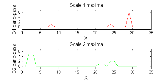
red=double(X)-double(Y1);
green=double(Y1)-double(Y2);
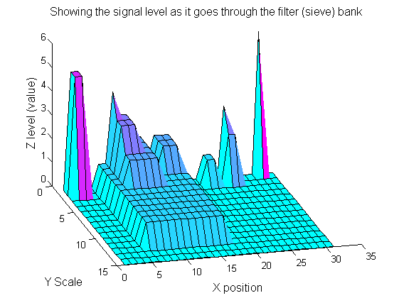
Repeat over scales 0 to 15
| Increasing the scale removes extrema of increasing length. | 
|
YY=ones([length(X),1+maxscale]);
for scale=0:maxscale
    Y2=SIVND_m(Y1,scale,'o',1,'l',4);
    YY(:,scale+1)=Y2';
    Y1=Y2; % each stage of the filter (sieve) is idempotent
end


