"Evolution through genetically controlled allometry space"

Downloading the Project and AAMToolbox
The project used to create the figures in the manuscript, together with the Matlab toolbox that manages the project can be downloaded here. (This contains version 6.5 of the AAMToolbox) File:Langlade 2005 PNAS.pdf To create the figures shown in the manuscript “Evolution through genetically controlled allometry space”, N. B. Langlade, X. Feng, T. Dransfield, L. Copsy, A. I. Hanna, C. Thebaud, J. A. Bangham, A. Hudson, and E. S. Coen, PNAS, 2005, please follow the instructions below.
These figures were created using Matlab 2006b version 7.3.0.267 running on Windows XP.
Installing the AAMToolbox
To install the toolbox, simply unzip the zip file you downloaded from the section above. In that folder you will find 2 folders, the first one will be the ‘AAMToolbox’ folder (this contains the Matlab files that run the toolbox). The second folder is named ‘PRJ_PNAS2005’. This is the project folder that contains all the data for the manuscript. To install the toolbox, from the Matlab prompt type
>>pathtool
Click the ‘Add with subfolders’ button and then select the AAMToolbox folder. Save your new path and return to Matlab. You have now installed the toolbox. REMEMBER, ANY CHANGES YOU MAKE TO THE TOOLBOX DIRECTORY WILL REQUIRE YOU TO RESET THE PATH USING PATHOOL.
Recreating Figures
Figure 1
This is an image available for download.
Figure 2
From the Matlab prompt type
>>figure_1_points_around_leaf
And select LE19.temp_dat from the Templates directory. The colours are your choice.
Figure 3
From the Matlab prompt type
>>figure_2_pc_effects
- Select the folder ‘PRJ_PNAS2005\StatisticalModels\LE19\Set_1\ImageList_1’ for the model (not scaled).
- Next choose the PCs you want to display (1 to 3 in our case).
- Next choose to use the mean from the model and finally select 2SD range. (The vertical and horizontal ranges can be changed but the default gets you started).
Figure 4
From the Matlab prompt type
>>AAMToolbox
- Make sure that the current model is LE19\Set_1\ImageList_1 from the drop down list.
- Next click the View Shape Space button.
- Next click the Open button from the Groups panel and select Majus_Charidemi_Groups.
- Next click the Load button from the Groups panel.
- Next select ‘Tools-Units-Standard Deviations’.
- Next uncheck Group Labels, Group Means, Particles from the plot options panel.
- Next check Ellipses and Vectors from the plot options panel.
- Next click the Choose Shape Axes button and select the PCs 1, 2, and 3.
- Next select Import from the Vectors menu and select QTL_Vectors.xls.
- (Optional) Select Walk from the Vectors to walk along the vectors.
Figure 5 (a)
UNDER CONSTRUCTION
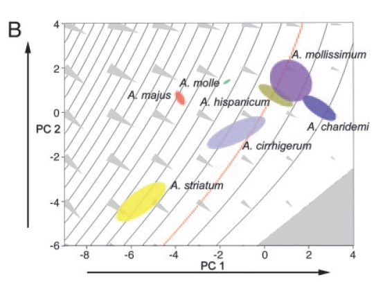
Figure 5 (b)
From the Matlab prompt type
>>AAMToolbox
- Make sure that the current model is LE19\Set_1\ImageList_1 from the drop down list.
- Next click the View Shape Space button.
- Next click the Open button from the Groups panel and select Species_Groups.mat.
- Next click the Load button from the Groups panel.
- Next select ‘Tools-Units-Standard Deviations’.
- Next uncheck Group Labels, Group Means, Particles from the plot options panel.
- Next check Ellipses from the plot options panel.
- Next click the Choose Shape Axes button and select the PCs 1, 2, and 3.
Figure 6
THESE FIGURES WERE CREATED WITH A TOOL NOT AVAILABLE FOR DOWNLOAD