"Evo"
Downloading the Project and AAMToolbox
The project used to create the figures in the manuscript, together with the Matlab toolbox that manages the project can be downloaded here. (This contains version 6.5 of the AAMToolbox)
To create the figures shown in the manuscript “Mutational spaces for leaf shape and size”, S. Bensmihen, A. I. Hanna, N. B. Langlade, J. L. Micol, A. Bangham, and E. S. Coen, HFSP Journal, 2008, please follow the instructions below.
These figures were created using Matlab 2006b version 7.3.0.267 running on Windows XP.
Installing the AAMToolbox
To install the toolbox, simply unzip the zip file you downloaded from the section above. In that folder you will find 2 folders, the first one will be the ‘AAMToolbox’ folder (this contains the Matlab files that run the toolbox). The second folder is named ‘PRJ_Arabid_Antirrh’. This is the project folder that contains all the data for the manuscript. To install the toolbox, from the Matlab prompt type
>>pathtool
Click the ‘Add with subfolders’ button and then select the AAMToolbox folder. Save your new path and return to Matlab. You have now installed the toolbox. REMEMBER, ANY CHANGES YOU MAKE TO THE TOOLBOX DIRECTORY WILL REQUIRE YOU TO RESET THE PATH USING PATHOOL.
Creating Figures
Figure 1
From the Matlab prompt type
>>figure_1_points_around_leaf
And select LE50template_04_05_06.temp_dat from the Templates directory. The colours are your choice.
Figure 2
From the Matlab prompt type
>>figure_2_pc_effects
- Select the folder ‘PRJ_Arabid_Antirrh\StatisticalModels\LE50Template_04_05_06\Set_1\ImageList_18’ for model (Ler only, not scaled).
- Next choose the PCs you want to display (1 to 5 in our case).
- Next choose to use the mean from the model and finally select 2SD range. (The vertical and horizontal ranges can be changed but the default gets you started).
Figure 3
From the Matlab prompt type
>>AAMToolbox
- Make sure that the current model is “LE50Template_04_05_06\Set_1\ImageList_18” from the drop down list.
- Next click the “View Shape Space” button.
- Next click the “Open” button from the Groups panel and select “all_groups_no_tsk”.
- Next click the “Load” button from the Groups panel.
- Next select ‘Tools-Units-Standard Deviations’.
- Next uncheck the “Group Labels” from the plot options panel.
- Next click the “Choose Shape Axes” button and select the PC 1. (To view another PC click the “Choose Shape Axes” button and choose the PC of interest (in our case PC1, PC2, PC3, PC4).)
Figure 4
UNDER CONSTRUCTION
Figure 5
From the Matlab prompt type
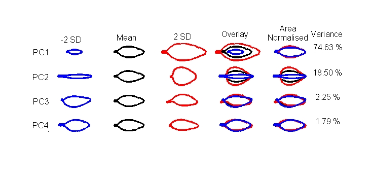
>>figure_2_pc_effects
- Select the folder ‘PRJ_Arabid_Antirrh\StatisticalModels\LE50Template_04_05_06\Set_1\ImageList_17’ for model (Ler only, scaled).
- Next choose the PCs you want to display (1 to 4 in our case).
- Next choose to use the mean from the model and finally select 2SD range. (The vertical and horizontal ranges can be changed but the default gets you started).
Figure 6
From the Matlab prompt type
>>figure_2_pc_effects
- Select the folder ‘PRJ_Arabid_Antirrh\StatisticalModels\LE50Template_04_05_06\Set_1\ImageList_21’ for model (_epure= cleaned form double mutant and flower effect mutants).
- Next choose the PCs you want to display (1 to 4 in our case).
- Next choose to use the mean from the model and finally select 2SD range. (The vertical and horizontal ranges can be changed but the default gets you started).
Figure 7
UNDER CONSTRUCTION
Figure 8
From the Matlab prompt type
>>AAMToolbox
- Make sure that the current model is “LE50Template LE50Template_04_05_06\Set_1\ImageList_21” from the drop down list.
- Next click the “View Shape Space” button.
- Next click the “Open” button from the Groups panel and select “ran_re _double”.
- Next click the “Load” button from the Groups panel.
- Next click the “Choose Shape Axes” button.
- Next select PCs 1 and 2 and hit “Ok”
- Next uncheck “Particles” and “Group Labels” from the “Plot Options” panel.
(The leaf pictures originated from the original pictures (observed). Vectors were added in the Adobe Illustrator CS2 software)
Figure 9
- Top panel: the outlines of young and mature Arabidopsis and antirrhinum leaves from Yvette’s pictures (for Munderman et al.?) were cut and filled (using the magic stick from Adobe Photoshop). Pictures were copied to Adobe Illustrator CS2 and scaled (selecting your shape, using then from the bar menu: object, transformation, scaling (“mise à l’échelle” in the French version).
- Bottom panel: the outlines of the Arabidopsis and Antirrhinum mean shapes, plus or minus 2SD, were created using the figure_2_pc_effects script as described for Figure 2. The file was saved as .eps and opened in Adobe Illustrator CS2 and the same scaling procedure was used.
Creating Tables
- Table 1 originates from the ranked t-test analysis described above performed on all the Arabidopsis Ler groups (on Image List 18 model). Groups were arranged and sorted in XL.
- Table 2 originates from the ranked t-test analysis (from Image List 21 model) of the antirrhinum groups (E_groups) using as wild type a group of 3 flower mutant groups (“flower_only_formean” group).
