Back to Tutorial pages
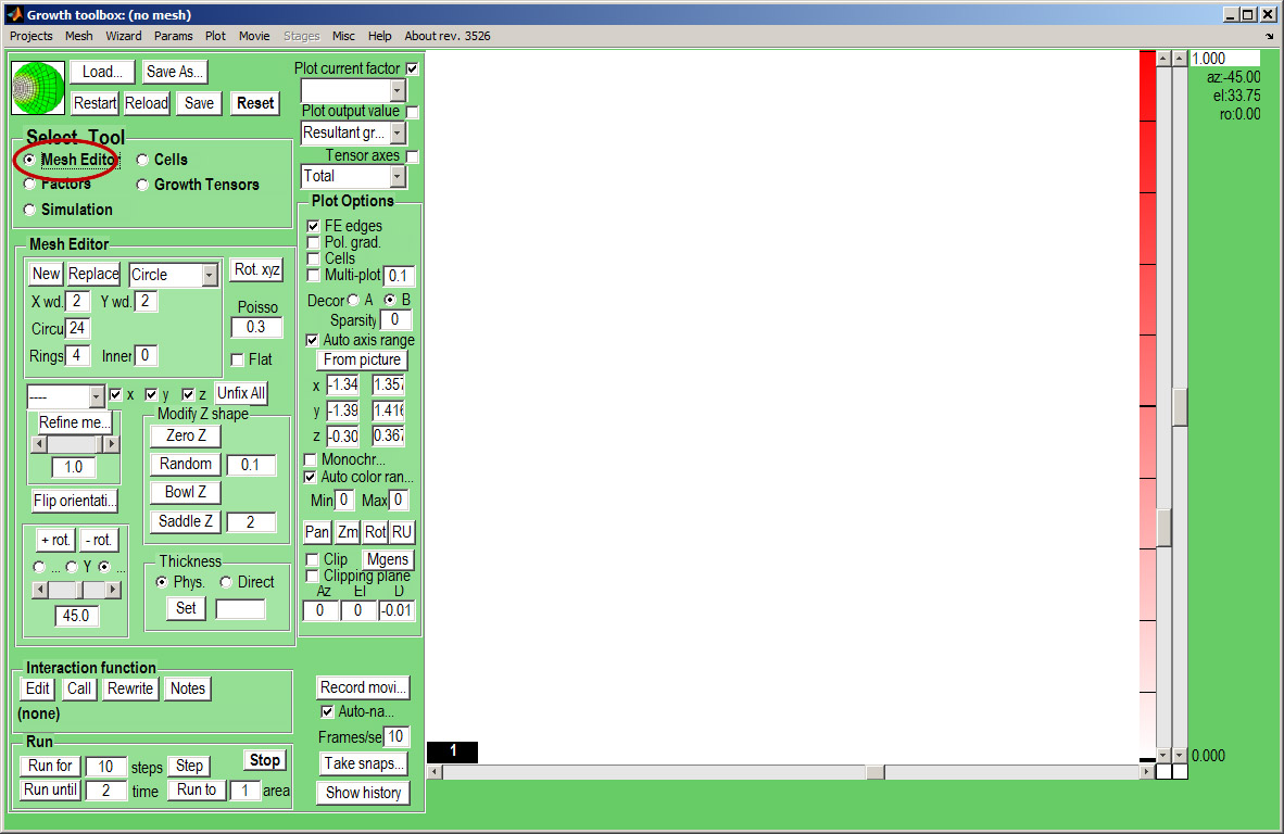
We start with a number of very large screenshots (don't be daunted they are just here to orient you). They show the GFtbox graphical interface.
Modelling non-uniform growth using the GUI alone
First view
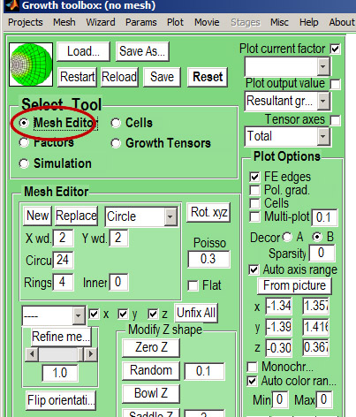
The GFtbox user interface. Focus on the Select Tool Panel. Here the Mesh Editor has been selected and the Mesh Editor panel is visible.

Idea: change all GFtbox font sizes using Menu Misc:Gui Format
|

|
Add a mesh (canvas that represents tissue)
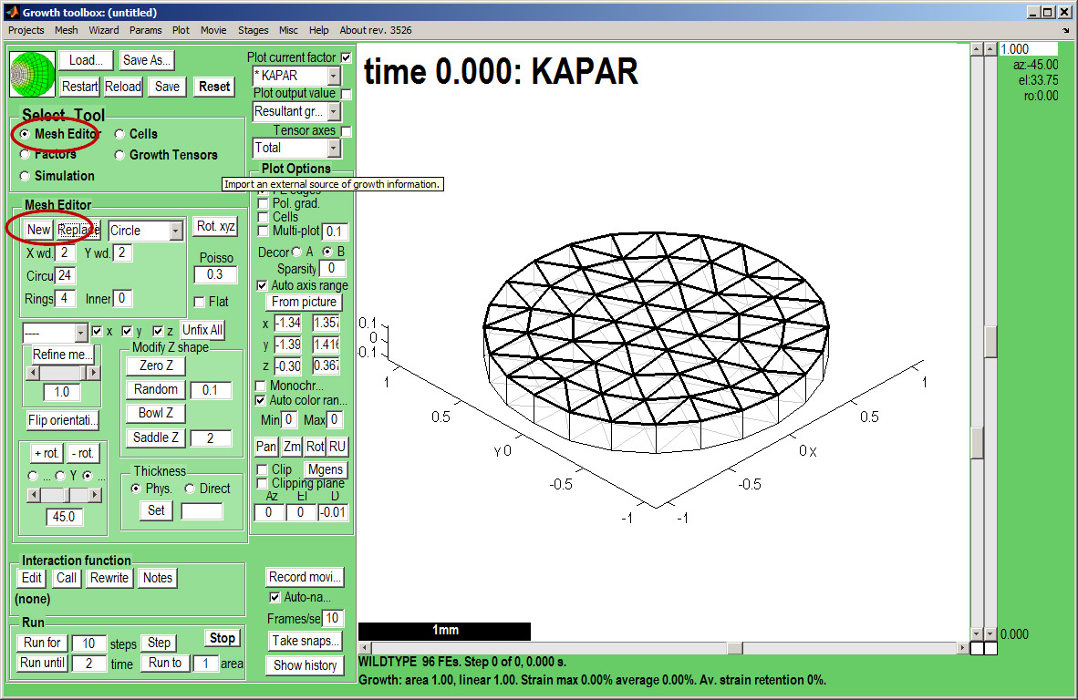
Create a canvas by clicking on Panel Mesh Editor:new. A variety of preset shapes are available, here we choose a Circle with 4 concentric rings of nodes that is 2 mm in diameter.
Idea: Special shapes can be imported as OBJ files.
|

|
Add a pattern of growth factor
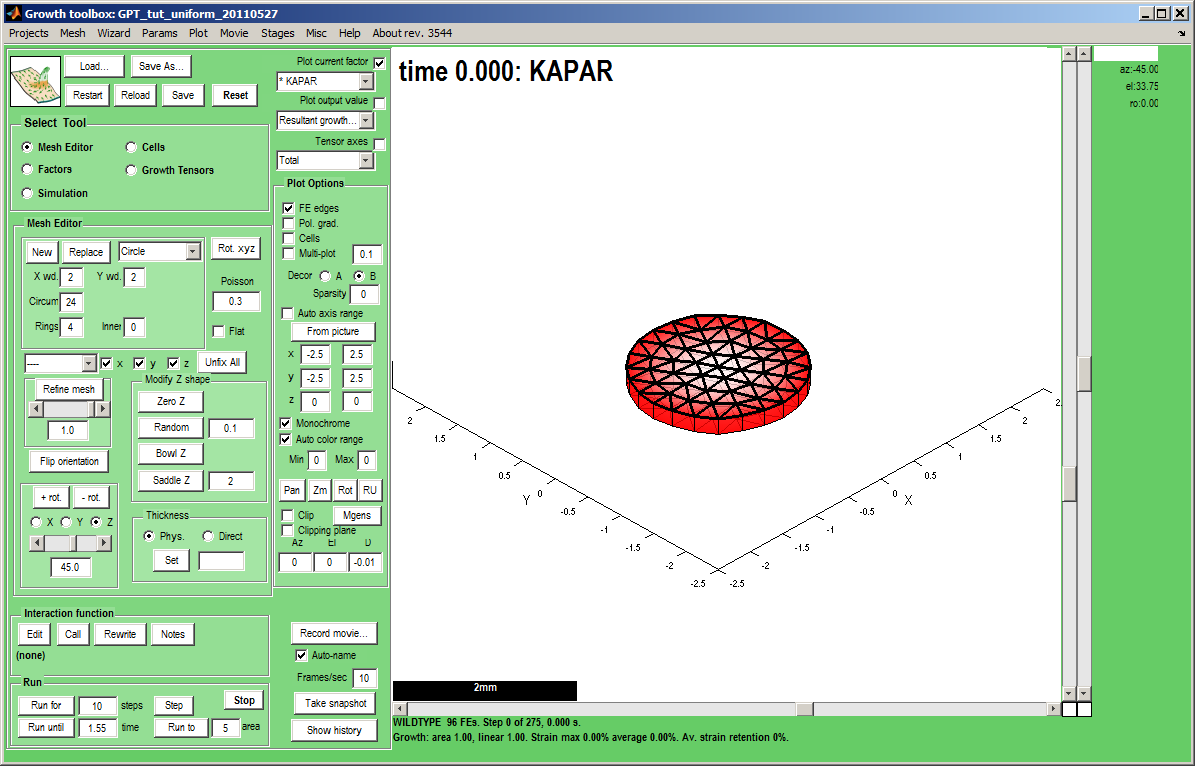
Select Tool:Factors makes the Morphogen Panel visible. Currently we are controlling the KAPAR factor. It has been selected from a drop down list top right (Plot current factor). We add a radially increasing gradient of KAPAR. Make sure that the Panel Plot Options:Monochrome is ticked and the gradient of KAPAR will be as shown. Do the same for the top face, KBPAR.
What will be the result of growth on just the bottom side of the canvas, KAPAR?
Note: the different ways to fix the levels of morphogens - 'Add constant', 'Add random', 'Add to rim', 'Add radial' centred on x,y,z position, 'Add linear'. In addition, if Panel: Plot Options: FE edges is ticked to reveal the mesh, clicking on a node will add the specified amount (slider) to that node alone. To set values (as opposed to adding) use 'Set zero' or select 'Set' in the list box.
Colours are set by clicking on the colour boxes.
|

|
And grow
Now save the project using the Save As button. A dialogue box will open - here we keyed in in_the_beginning and the prefix GPT_ and the suffix _date was added automatically.
A directory is created with the project name which contains all the files needed for the project and any results (snapshots, movies) we create.
Select Tool:Simulation makes the Simulation Panel visible.
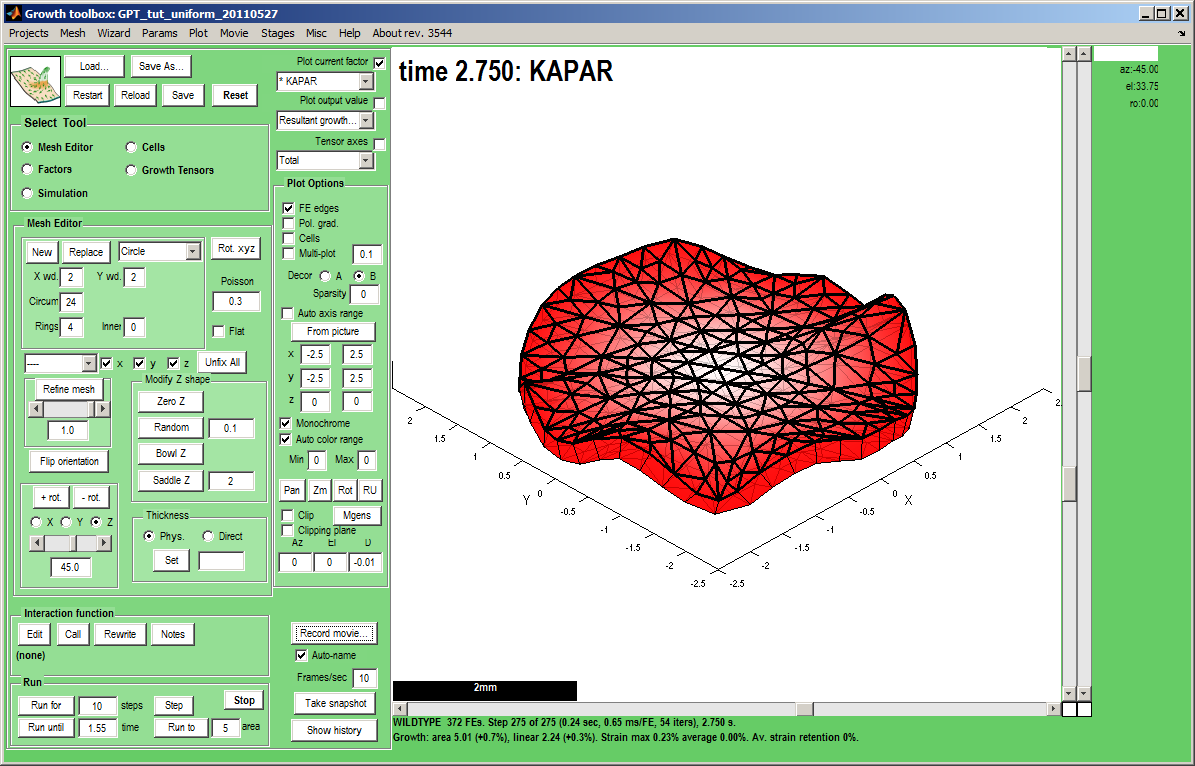
Change the Panel Run:Run until box to 2 and click the Panel Run:Run until button. The canvas will grow in steps set by the Panel Simulation:Timescale box.
Warning: saving is essential if you want to Restart the simulation.
Idea: set the axes manually (here to +-3) and turn off Panel:Plot Options: Auto axis range and Menu:Plot:Auto zoom and centre. This enables growth to be seen as a change of size rather than change of axis range.
Idea: take a snapshot of the canvas by pressing Take snap... (c.f. image on right, button is bottom right of GUI controls)
Idea: to create an uncompressed movie of your simulation, before running click the Record movie and when it is finished click Stop movie. The movie will be in the Project directory. Compressors can be selected using the Menu: Movie: Codec option and the result can be converted to a flash movie (for the web) by Menu: Movie: Convert to flash this, however, requires ffmpeg to be installed on the computer.
|
 Extra growth around the perimeter introduces Gaussian curvature. The canvas is readily able to distort out the plane because it started out with a small amount of random noise in the Z direction. (If the canvas started perfectly flat, residual strain (stress) would build up at each step rather than the surface distorting to accommodate the extra growth.) Extra growth around the perimeter introduces Gaussian curvature. The canvas is readily able to distort out the plane because it started out with a small amount of random noise in the Z direction. (If the canvas started perfectly flat, residual strain (stress) would build up at each step rather than the surface distorting to accommodate the extra growth.)
|
