GFtbox Tutorial pages

GFtbox Details
Notes from a new user
Running example models and using a cluster
Examples from our papers
Types of morphogens and factors are given here
(A newly created interaction function is shown here - the green comments are another ready reference.)
Ready Reference Manual

The models shown in these tutorials illustrate features of the GFtbox software. They are not designed to understand the Growing Polarised Tissue Framework which is better done with Examples from our papers.

Viewing these pages. Some versions of Firefox and Explorer do not create satisfactory prints even though you can view the pages with no problems. Chrome does appear to produce good printouts.

Three ways to use GFtbox

1) Do everything from the Graphical User Interface (GUI).

2) Do only some things from the GUI. Use the GUI to generate the mesh (canvas) and create growth factors, but capturing your ideas on how the regulatory processes work by writing Matlab code in what we call the interaction function.

3) Without the GUI. For example, run many examples (instances) of a pre-existing project on a cluster. This is the best way to explore the parameter space of a model for comparison with biological observations. We use this extensively once we have roughed out the basic ideas of a model interactively.

Hints and Tips

1. Ready Reference Manual worth printing it includes details on taking snapshots and movies (and solving problems)
2. Multiple Figures for publication colours and viewpoints.
3. Movies for publication and web codecs compression and Powerpoint.
4. Quality and accuracy
   1. Mesh: tradeoff between memory/speed and accuracy. Increasing the number of vertices in specific regions
   2. Time: tradeoff between speed and accuracy. Checking that time steps are small enough.
   3. Tolerances: tradeoff between speed and accuracy. Checking that tolerances are tight enough.
5. Measuring model growth
   1. Measuring using interaction function subroutines
6. Mesh: cutting and flattening Dissecting a mesh and flattening the parts

1 Modelling using the Graphical User Interface

Isotropic growth

How to use the tutorial. Open GFtbox and attempt to repeat the results shown.

1 A

Tutorial on uniform growth. Consider a disc shaped canvas (tissue) in which the specified growth is uniform, isotropic and on both sides. Into what shape will the disc grow? This model is as simple as it gets. Notice that, during growth, the mesh is automatically subdivided. Notice also that the final surface is not quite flat. This is because, to allow it to deform in 3D, it is not flat initially. There are options to initialise a flat mesh and others to force it to remain flat - see options on the GUI (hover over controls to get prompts). In the absence of a polariser (there is no polariser in this example) growth will be isotropic, in other words growth in the plane of the canvas will be the average of what is specified for Kapar and Kaper (A side) and Kbpar and Kbper (B side).

<wikiflv width="300" height="300" logo="false" loop="true" background="white">GPT_tut_uniform_20110527-0003.flv|GPT_tut_uniform_20110527-0003_Last.png</wikiflv>

1 B

Tutorial on non-uniform growth. Consider a disc shaped canvas (tissue) in which the non-uniform specified growth increases in proportion to the distance from the centre. Into what shape will the disc grow? Already we are into the realms of modelling biological systems. Compare this result with the discussion of Lily petals and Gaussian curvature (Lianga and Mahadevana,Sharon, Marder and Swinney,Nath, Crawford, Carpenter and Coen ).

<wikiflv width="300" height="300" logo="false" loop="true" background="white">GPT_tut_uniform_20110527-0006.flv|GPT_tut_uniform_20110527-0006_First.png</wikiflv>

Adding polariser

1 C

Tutorial on uniform growth with non-uniform polariser. In the presence of polariser, GFtbox growth will be anisotropic, in other words growth in the plane of the canvas can be different parallel and perpendicular to the axis of the polariser: Kapar and Kaper (A side) and Kbpar and Kbper (B side). We now add polariser. Start with example A - uniform growth - and add a radial polarising gradient. Arrows show the direction of the gradient. They are turned on using the Panel:Plot option:Pol. grad. tick box. The gradient defines local directions and local growth can be specifed either parallel to (Kpar) or perpendicular to (Kper) that direction. Given a uniform pattern of specified growth parallel to the polariser and zero specified growth perpendicular to the polariser. What will be the final shape? Note: the gradient of the polariser, green to cyan, is shown using the arrows. Specified growth rate parallel to the arrows, red, is uniform.

<wikiflv width="300" height="300" logo="false" loop="true" background="white">GPT_in_the_beginning_2_20110510-0003.flv|GPT_in_the_beginning_2_20110510-0003_First.png</wikiflv>

2 Modelling using a combination of GUI and interaction function

How to use these tutorials. Use a combination of the GUI to set up the Mesh structure and editing the associated interaction function to repeat the results shown. Full listings of the interaction functions are given from which you can copy the key, editable, elements.

The full specification of a GFtbox model is stored in a combination of the mesh data structure (Mesh) and the interaction function. The Mesh stores all the physical properties of the system: spatial structure, mechanical properties, etc. It is usually set up using the GUI. The Mesh is stored on disc as a Matlab data file (.mat) and in memory as a data structure (m). The interaction function (a Matlab program file .m) contains all the details of the growth regulation system: morphogen concentrations, signal interactions etc.

When a new project is first edited the interaction function is generated automatically. Thereafter, it is automatically kept in synchrony with the GUI. It is divided into several sections. Some are generated automatically and should not be edited. Others are set aside for the user to specify the model. To ensure that the automatic and manual edits are synchronised always invoke the Editor from the GUI (Panel: Interaction Function: Edit).

2 A

Basic interaction function The patterns of morphogens A and B are set up by

       id_a_p(m.nodes(:,1) < -0.03) = 1; 
       id_b_p(m.nodes(:,2) < -0.01) = 1; 

where id_a_p is the A morphogen. m.node(:,1) refers to the x coordinates of all nodes (vertices) in the mesh
The expression (m.nodes(:,1) < -0.03) means find all vertices with x coordinates that are less than -0.03.

Similarly, (m.nodes(:,2) < -0.01) means find all vertices with y coordinates that are less than -0.01.

And the pattern of polariser (P) is set up by

       P((m.nodes(:,1) < -0.05) & (m.nodes(:,2) > 0.03)) = 1;

Where (m.nodes(:,1) < -0.05) & (m.nodes(:,2) > 0.03) means find all vertices with x,y coordinates that are less than -0.05 and greater than 0.03 respectively

Thus the full code describing the model is:

   if (Steps(m)==0) && m.globalDynamicProps.doinit  % Initialisation code.
       id_a_p(m.nodes(:,1) < -0.03) = 1; % setup region for A where identity factor A is represented by id_a_p
       id_b_p(m.nodes(:,2) < -0.01) = 1; % setup region for B
   else
       % @@KRN Growth Regulatory Network
       kapar_p(:) = id_a_l .* inh(1,id_b_l); % growth rate
       kaper_p(:) = kapar_p; % isotropic growth
       kbpar_p(:) = kapar_p; % same on both sides of the sheet
       kbper_p(:) = kapar_p; % same
       knor_p(:)  = 0;       % thickness not growing
   end

Tutorial on a basic interaction function. The tutorial explains how the code shown above appears in the interaction function. To create the interaction function, first create and save a project (see above) then click Panel:Interaction function:Edit. The interaction function will contain all the default variables and any patterns of variables (Kapar, etc.) that have already been set through the GUI. Types of morphogens and factors are given here.

<wikiflv width="300" height="300" logo="false" loop="true">GPT_why_matlab-2011-05-05-0005.flv|GPT_why_matlab-2011-05-05-0005_First.png‎</wikiflv>

Play and the mesh will grow and subdivide. Normally we do not want to see the mesh. Red is growth rate

2 B

Interaction function in detail

(A newly created interaction function is shown here - this one has two, user specified morphogens: id_a and id_b.)

There are two submodels. An identical growth pattern and polariser pattern is specified in both, but only the specified growth in the second is anisotropic and so uses the axiality specified by the polariser gradient. The gradient is zero in the region where the polariser is held at a constant value of one - and therefore growth in the region without arrows is isotropic.

Tutorial on the interaction function details. Types of morphogens and factors are given here. Submodel 1	<wikiflv width="300" height="300" logo="false" loop="true">GPT_tut_interaction_example_20110601-0002.flv|GPT_tut_interaction_example_20110601-0002.png‎</wikiflv>
Submodel 2. Growth in the region that has no arrows is isotropic and, as result, the outgrowth is blunt.	<wikiflv width="300" height="300" logo="false" loop="true">GPT_tut_interaction_example_20110601-0007.flv|GPT_tut_interaction_example_20110601-0006_Last.png‎</wikiflv>

2 C Illustrating independent ways to form shapes and the use of submodels.

Conclusion: interesting shapes can be generated either by patterns of differential growth or patterns of local growth axes.

Tutorial on different ways of specifying the growth of shapes.

Submodel 1. Uniform specified polariser (no polariser gradient). Creating a shape using a specified pattern of isotropic growth. Result: simple patterns of differential growth can readily produce blobby shapes.	<wikiflv width="300" height="300" logo="false" loop="true">GPT_TwoWayHeart_20110531-0001.flv|GPT_TwoWayHeart_20110531-0001_Last.png‎</wikiflv> Play submodel 1. Pattern of isotropic specified growth (no polariser)
Submodel 2.Uniform specified growth. Creating a shape using a specified pattern of diffusable polariser. Result: simple patterns organising a diffusable polariser can readily produce sharp shapes. Outputs from these models bear only a romantic relation to hearts, flowers and lepidoptra.	<wikiflv width="300" height="300" logo="false" loop="true">GPT_TwoWayHeart_20110531-0002.flv|GPT_TwoWayHeart_20110531-0002_Last.png‎</wikiflv> Play submodel 2. Pattern of specified polariser levels (green-cyan). Polariser can diffuse and the gradient is arrowed. Uniform specified growth (red).

2 D

Retaining strain and cutting the mesh

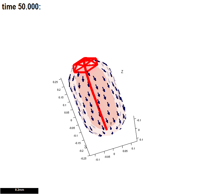
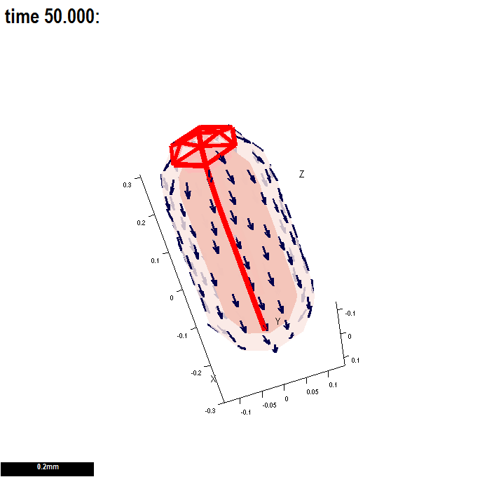
There are two submodels. They are the same except that in the first strain is not retained from step to step whereas in the second strain is fully retained. The shape changes during growth look similar, the difference is only revealed when the mesh is cut. The behaviour of plant tissue can be similar.

Tutorial on retaining residual strain and cutting

Strain not retained after each step. In plant tissue terms this would appear to be equivalent to there being a homeostatic mechanism that operates such as to re-strengthen the cell walls after they have been weakened to the point that they yield under turgor pressure during growth.	<wikiflv width="300" height="300" logo="false" loop="true">GPT_RetainStrainAndCut_20110603-0006.flv|GPT_RetainStrainAndCut_20110603-0006.png‎</wikiflv> Play submodel 1
Retaining the strain from step to step allows the growth on the inside to force the mesh as a whole to grow more than when strain is not retained.	<wikiflv width="300" height="300" logo="false" loop="true">GPT_RetainStrainAndCut_20110603-0004.flv|GPT_RetainStrainAndCut_20110603-0004.png‎</wikiflv> Whilst the frame rate relates directly to growth rate, the relaxation rate after cutting does not. After cutting the computation has to be done in smaller steps and the rate at which the sides bend back shown here is too slow.

3 Cluster runs and batch mode: running models without the GUI

Having developed the concepts underpinning a pattern of growth in an interaction function it is often desirable to explore a range of model parameters. Given that each run of the model can take between 5 minutes and hour it is appropriate to run the models in batch mode on the desktop or, better, in parallel on a computing cluster. (Each node of the cluster to be used by GFtbox needs to be licensed to run Matlab - however for the purpose of running on a cluster without the GUI we are exploring the possibility of making GFtbox compatible with Octave.)

Batch mode and cluster runs.
How to use these tutorials. First ensure that your model is working as you would expect using the GUI. Then run the model from the Matlab command line. Finally, run the models in batch mode or submit the project to the linux computing cluster with one or more ranges of parameters. For further details Running example models and using a cluster

4 Comparing resultant shapes with observed organ shapes

4 A

Tutorial on mapping results into shape space

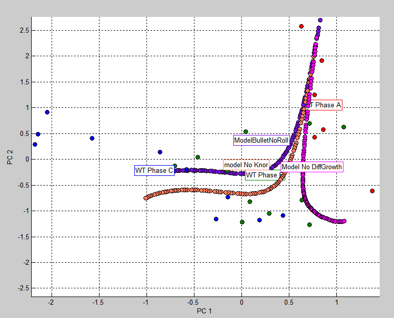<wikiflv width="300" height="300" logo="false" loop="true">GPT_tut_interaction_example_20110601-0002.flv|GPT_tut_interaction_example_20110601-0002.png‎</wikiflv> <left>(Marks) The shape of growing Arabidopsis leaves projected into a shape space represented by the two principal components. (Lines) The shape of a computational model of a growing Arabidopsis leaf projected into the same space.